Julia syntax basics – NeuroBorder

1 Julia pros and cons

1.1 Pros

Interactive programming

Julia is a dynamically typed language, in contrast with statically typed languages.

High performance

Julia uses just-in-time compilation (JIT), compilation at run time.

Typically, JIT continuously analyses the code being executed and identifies parts of the code where the speedup gained from compilation or recompilation would outweigh the overhead of compiling that code.

Therefore, JIT combines advantages of ahead-of-time compilation (AOT, compilation before execution) and interpretation.

Due to the ecosystem of packages, Julia is really suitable for scientific computing, but it can also be used as a general-purpose programming language.

1.2 Cons

Julia starts more slowly than Python, R, etc. but begins to run faster once the JIT compiler has converted critical parts of the code to machine code; thus it’s not suitable for:

Programming small, short-running scripts.
Real-time systems (Julia implements automatic garbage collection, which tends to introduce small random delays).
System programming (it needs detailed control of resource usage).
Embedded systems with limited memory.

2 Basics

2.1 Arithmetic operations and number types

2.1.1 Arithmetic operations

Addition, subtraction, multiplication, division, and power: + - * / ^.

2.1.2 Number types

Signed integers: Int8, Int16, Int32, Int64 (default), Int128, BigInt.
Unsigned integers: UInt8, UInt16, UInt32, UInt64, UInt128.

You can check the minimum and maximum values of a certain integer type with typemin() and typemax().

You can check the type of the input argument with typeof().

Julia defaults to showing all signed integers in decimal format, and all unsigned integers in hexadecimal format.

In fact, what is stored in memory is no difference. The only difference is how to interpret it. You can use the reinterpret() function to see how the exactly same bits in memory can be interpreted differently.

Floating-point numbers: Float16, Float32, Float64 (default).

You can type a Float32 number by suffixing f0: 3.14f0.

Rational type: 2 // 5 represents a rational number $\frac{2}{5}$.
Complex type: 1 + 2im.

2.1.3 Arithmetic operations for integers

/ always gives floating-point number

4 / 2

2.0

÷ or div() gives the quotient

5 ÷ 3

div(5, 3)

% or rem() gives the remainder

5 % 3

rem(5, 3)

divrem() gives both quotient and remainder

divrem(5, 3)

(1, 2)

Caution

Typically, operations on the same type of values always give the same type of value, even though overflow may occur.

Even though overflow will occur, Julia won’t give any prompt.

2.2 Variables

In julia, identifiers can be used to give names to constants, variables, types, and functions.

Variables defining memory addresses where values are stored, are only references to values, because Julia allocates memory based on values, not variables.

In comparison with this, statically typed languages allocate memory based on variables, so you must first decalre the type of a variable (e.g., int) before using it, which will allocate a predefined size (which depends on the type of the variable) in a predefined location in memory to this variable. As a consequence, you should never attempt to assign a value that cannot fit inside the memory slot set aside for the variable to this variable.

The equal sign (=) operator is used to assign values to variables (i.e., let a variable point to a value):

x = 1

Allowed variable names:

Leading characters: letters, underscore, Unicode code points greater than 00A0.
Subsequent characters: other Unicode code points.
Variable names containing only underscores can only be assigned values, which are immediately discarded.
Explicitly disallowed variable names: built-in keywords.

Tip

To type many special characters, like Unicode math symbols, you can type the backslashed LaTeX symbol name followed by tab.

If you find a symbol elsewhere, which you don’t know how to type, the REPL help will tell you: just type ? and then paste the symbol.

My own rules for clarity:

Can only contain letters, underscore, and numbers.
Can only start with letters.

Two special variables:

Constants: defined with the const keyword.

const my_pi = 3.14

3.14

Note

You can still assign a new value with the same type as the original one to a constant, but a warning is printed.

The ans variable: in interactive mode, Julia REPL assigns the value of the last expression to the ans (answer) variable.

Literal coefficient

In mathematics, 3×x + 2×y may be written as 3x + 2y. Julia lets you write a multiplication in the same manner. We refer to this as literal coefficient, which is a shorthand for multiplication between a number literal and a constant or variable:

x = 3
2x

2*(3+2)
2(3+2)

2*π
2π

2.3 Relation and logical operations

2.3.1 Relation operations

==, != or ≠, <, >, <= or ≤, >= or ≥

The operation result is true or false, which is Bool type.

2.3.2 Logical operations

&&, ||, !

The logical evaluation is lazy.

Suppose i = 10, and then 1 <= i <= 100 is equivalent to i >= 1 && i <= 100.

2.4 Control flow

2.4.1 Comment

In Julial, you can give an inline comment by using #, or multiline comment by using #=...=#.

2.4.2 Compound expressions

To have a single expression which evaluates several subexpressions in order, returning the value of the last subexpression as its value.

; chain

Put all subexpressions separated by ; inside parentheses.

z = (x = 1; y = 2; x + y)

# or
z = (x = 1;
     y = 2;
     x + y)

z

begin block

Put all subexpressions separated by a newline character between begin and end keywords.

You can also put all subexpressions in one line by separating them with ;.

z = begin
    x = 1
    y = 2
    x + y
    end

# or
z = begin x = 1; y = 2; x + y end

z

This is quite useful for the inline function definition.

Note

For multiple statements, you can put them in one line and separate them with ;, which is not the same thing as compound expressions:

x = 1 + 2; println("x=$x")

x=3

2.4.3 Short-circuit evaluation

cond && expr: evaluate expr if and only if cond is true.
cond || expr: evaluate expr if and only if cond is false.

2.4.4 Conditional evaluation

if cond1
    statements
elseif cond2
    statements
...
else
    statements
end

Note

Ternary operator: cond ? expr1 : expr2, which is closely equivalent to if cond expr1 else expr2.

2.4.5 Looping

while

while cond
    statements
end

‘for’

for var in iterable
    statements
end

For for loop, var in iterable, var ∈ iterable, and var = iterable are equivalent to one another!

Note 1: Member operator in or ∈

in(collection) or ∈(collection) creates a function which checks whether its argument is in collection:

f = in(1:10)

f(1)

true

Note: start:stop will generate a number sequence with step 1; start:step:stop with step step.

in(item, collection) or ∈(item, collection) determines whether an item is in the given collection:

in(1, 1:10)

true

Sets check whether the item is equal to one of the elements:

1 in Set(1:10)

true

Dicts look for key=>value pairs:

(1=>10) in Dict(1=>10, 2=>20)

true

in.(items, collection) or items .∈ collection checks whether each value in items and each value in collection at the corresponding position are the same one:

If either items or collection contains only one element, it will be broadcasted to the same length as the longer.

in.([1, 3, 2], [1, 4, 2])

3-element BitVector:
 1
 0
 1

in.(items, Ref(collection)) or items .∈ Ref(collection) checks whether each value in items is in collection:

Ref(collection) can also be written as (collection,) (i.e. wrap collection in a tuple or a Ref).

Note: create a tuple containing only one element with (1,).

in.([1, 3, 2], Ref([8, 6, 1, 4, 3, 2]))

3-element BitVector:
 1
 1
 1

in. does not support infix form!

in, ∈, and .∈ support both forms!

In contrary to ∈ (\in<tab>), ∋ (\ni<tab>), and .∈, we have, ∉ (\notin<tab>), ∌ (\nni<tab>), and .∉.

2.4.6 Jump out of loops

break: jump out of the loop in which break is.
continue: stop an iteration and move on to the next one.
@goto name and @label name: @goto name unconditionally jumps to the statement at the location @label name.

2.5 Functions

2.5.1 Inline functions

<function name>(<parameters>) = <expression>:

cylinder_volume(r, h) = π*r^2*h

cylinder_volume(5, 3)

235.61944901923448

2.5.2 Multiline functions

function <function name>(parameters)
    ...
end

In Julia, return <value> is not necessary. It is only used when you need to exit a function early; otherwise the value of the last expression will always be returned.

Note

Functions are central to Julia! Various interfaces are achieved by functions even though they don’t look like functions.

Infix form

5 + 3

Prefix form

+(5 + 3 + 5)

If a function with a symbol name takes two arguments, we can use it by infix form:

↔(x, y) = x^2 + y^2

6 ↔ 6

2.5.3 Argument passing behaviour

Pass-by-sharing!

2.5.4 Specify the type of return value

You can specify the type of return value of a function in the form FuncName(parameters)::ReturnType.

If the type of return value is not the given type, a conversion is attempted with convert().

foo(x::Int64) :: Int32 = 2x

typeof(foo(6))

Int32

2.5.5 Multiple assignments and multiple return values

Multiple assignments

Achieved by using (named) tuples.

(a, b, c) = 1:3  # Assign each variable a value; parentheses are optional

_, _, a = 1:3  # Use _ to discard unwanted values

a, b..., c = 1:6  # a -> 1, b -> 2:5, c -> 6; b... indicates that b is a collection (b doesn't need to be the final one)

(; b, a) = (a=1, b=2, c=3)  # Assign values to variables based on names

Multiple return values

2.5.6 Parameter types

Positional parameters: non-optional; optional with defaults.
Keyword parameters: non-optional; optional with defaults.

(a, b = 1; c, d = 2)  # Keyword arguments are defined after ;

# Positional arguments: a, b (optional)
# Keyword arguments: c, d (optional)

# When you pass arguments, either will be fine:
(1, 2; c = 3, d = 4)  # Separated by ;
(1, 2, c = 3, d = 4)  # Separated by ,

Important

Multiple dispatch only considers positional arguments.

2.5.7 Anonymous functions

Anonymous functions play an important role in functional programming.

An anonymous function can be defined in two ways:

Inline style: (<parameters>) -> <expression> (() can be omitted if it only has a single parameter).
Multiline style:

function (<parameters>)
    ...
end

2.5.7.1 `do` blocks

We can use do blocks to create mutiline anonymous functions.

The following two statements are equivalent:

map(x -> begin
              if x < 0 && iseven(x)
                  return 0
              elseif x == 0
                  return 1
              else
                  return x
              end
         end,
    [-2, 0, 2])

3-element Vector{Int64}:
 0
 1
 2

map([-2, 0, 2]) do x
    if x < 0 && iseven(x)
        return 0
    elseif x == 0
        return 1
    else
        return x
    end
end

3-element Vector{Int64}:
 0
 1
 2

In the above example, the do x syntax creates an anonymous function with argument x and passes it as the first argument to map().

Similarly, do x, y will create a two-argument anonymous function but do (x, y) will create a one-argument anonymous function, whose argument is a tuple.

In a word, we can use do blocks to create anonymous functions which are passed as the first argument to some higher-order functions, the first argument of which must be the Function type.

2.5.8 The splat operator `...`

The splat operator can be used to turn arrays or tuples into function arguments.

e.g. foo([1, 2, 3]...) is the same as foo(1, 2, 3).

You can define a parameter which accepts a variable number of arguments by using the splat operator:

# All arguments except the 1st will be stored in a tuple, assigned to args
function var_f(x, args...)
    ...
end

2.5.9 Closure

A closure is a function that has captured some external state not supplied as an argument since the inner scope can use variables defined in an outter scope.

Anonymous functions are frequently used as closures.

function make_pow(n::Real)  # Outer function
    function (x::Real)  # Inner function
        x^n  # The inner function uses n defined outside it and n is not passed as an argument to it
    end
end

pow2 = make_pow(2)  # The returned function with n=2 is assigned to variable pow2
pow3 = make_pow(3)

pow2(2), pow3(2)

(4, 8)

Performance of captured variable

For the consideration of performance, if the type of a captured variable is already known, you would better add a type annotation to it. In addition, if the value of this captured variable need not be changed after the closure is created, you can indicate it with a let block:

function abmult(r::Int)
    r1::Int = r  # Type annotation
    if r1 < 0
        r1 = -r1
    end
    f = let r1 = r1  # Fix it
            x -> x * r1
        end
    return f
end

f = abmult(10)
f(10)

2.5.10 Partial function application

Partial function application refers to the process of fixing a number of arguments to a function, producing another function accepting fewer arguments.

Obviously, closure is a way to achieve the partial function application.

2.5.11 Function composition, vectorization and piping

2.5.11.1 Function composition

The concept of function composition in Julia is the very concept of function composition in mathematics and the operation symbol is the same one: ∘, typed using \circ<tab> (e.g. (f ∘ g)(args...) is the same as f(g(args...))).

(sqrt ∘ +)(3, 6)  # Equivalent to sqrt(+(3, 6))

3.0

2.5.11.2 Dot syntax for vectorizing functions

In Julia, vectorized functions are not required for performance, and indeed it is often beneficial to write your own loops, but they can still be convenient.

You can add a dot . after regular function names (e.g. f) or before special operators (e.g. +) to get their vectorized versions.

Operating on a single array:

A = 1:3

sin.(A)  # Which is equivalent to map(sin, A) or broadcast(sin, A)

3-element Vector{Float64}:
 0.8414709848078965
 0.9092974268256817
 0.1411200080598672

Operating on multiple arrays (even of different shapes), or a mix of arrays and scalars:

fp(x, y) = 3x + 4y

A = 1:3
B = 4:6

fp.(pi, A)

3-element Vector{Float64}:
 13.42477796076938
 17.42477796076938
 21.42477796076938

fp.(A, B)

3-element Vector{Int64}:
 19
 26
 33

Keyword arguments are not broadcasted over, but are simply passed through to each of the function.
Nested f.(args...) calls are fused into a single broadcast loop.

X = 1:6

sin.(cos.(X))  # Equivalent to broadcast(x -> sin(cos(x)), X)

6-element Vector{Float64}:
  0.5143952585235492
 -0.4042391538522658
 -0.8360218615377305
 -0.6080830096407656
  0.2798733507685274
  0.819289219220601

However, the fusion stops as soon as a “non-dot” function call is encountered (e.g. sin.(sort(cos.(X)))).

The maximum efficiency is typically achieved when the output array of a vectorized operation is pre-alllocated.

X = 1:10000

@time sin.(X)

  0.000109 seconds (3 allocations: 78.203 KiB)

10000-element Vector{Float64}:
  0.8414709848078965
  0.9092974268256817
  0.1411200080598672
 -0.7568024953079282
 -0.9589242746631385
 -0.27941549819892586
  0.6569865987187891
  0.9893582466233818
  0.4121184852417566
 -0.5440211108893698
 -0.9999902065507035
 -0.5365729180004349
  0.4201670368266409
  ⋮
 -0.9534986003597155
 -0.26156028858731495
  0.6708553462651908
  0.9864896695694187
  0.39514994010172155
 -0.5594888219681838
 -0.9997361413354392
 -0.5208306628783247
  0.4369241250954582
  0.9929728874353159
  0.6360869563962336
 -0.30561438888825215

Y = Vector{Float64}(undef, 10000)  # Construct an uninitialized (undef) Vector{Float64} of length 10000

@time Y .= sin.(X)  # Overwrite Y with sin.(X) in-place

  0.010965 seconds (9.57 k allocations: 647.133 KiB, 98.74% compilation time)

10000-element Vector{Float64}:
  0.8414709848078965
  0.9092974268256817
  0.1411200080598672
 -0.7568024953079282
 -0.9589242746631385
 -0.27941549819892586
  0.6569865987187891
  0.9893582466233818
  0.4121184852417566
 -0.5440211108893698
 -0.9999902065507035
 -0.5365729180004349
  0.4201670368266409
  ⋮
 -0.9534986003597155
 -0.26156028858731495
  0.6708553462651908
  0.9864896695694187
  0.39514994010172155
 -0.5594888219681838
 -0.9997361413354392
 -0.5208306628783247
  0.4369241250954582
  0.9929728874353159
  0.6360869563962336
 -0.30561438888825215

Using the @. macro to convert every function call, operation, and assignment in an expression into the “dotted” version.

X = [1.0, 2.0, 3.0]

Y = similar(X)  # Pre-allocate the output array

@. Y = sin(cos(X))

3-element Vector{Float64}:
  0.5143952585235492
 -0.4042391538522658
 -0.8360218615377305

Using vectorized piping operator.

1:6 .|> [x -> x-1, inv, x -> 2*x, -, isodd, iseven]

6-element Vector{Real}:
    0
    0.5
    6
   -4
 true
 true

broadcast(f, As...)

Broadcast the function f over the arrays, tuples, collections, Refs, and/or scalars As.

Pre-allocating outputs

Vector{Int}(undef, 10)  # Construct an uninitialized Vector{Int} of length 10

10-element Vector{Int64}:
 125676241024704
 125687895638864
 125687925047304
 125687767111376
 125687925047304
 125687925047304
               1
              -1
               1
 125676226543626

Matrix{Float64}(undef, 3, 3)  # Construct an uninitialized Matrix{Float64} of 3 by 3

3×3 Matrix{Float64}:
 0.0  0.0  0.0
 0.0  0.0  0.0
 0.0  0.0  6.2098e-310

2.5.11.3 Function piping

The pipe operator is |>, which is used to chain together functions taking single arguments as inputs.

1:10 |> sum |> sqrt

7.416198487095663

2.6 Exception

Usage:

try
    <some code which may raise some errors>
catch <exception variable>
    <some code dealing with exceptions>
else
    <some code to be executed when no error occurs>
finally
    <some code to be executed anyway>
end

You can use throw() to raise a given type of exception or use error() to raise an ErrorException directly.

Then you can use isa() to check whether the error type raised is the expected.

e.g.

x = [2, -2, 'a']

for i in x
    try
        y = sqrt(i)
        println("√", i, " = ", y)
    catch e
        if isa(e, DomainError)
            println("√", i, ": $(i) is out of domain")
        else
            println("√", i, ": $(i) is an unsopported type")
        end
    end
end

√2 = 1.4142135623730951
√-2: -2 is out of domain
√a: a is an unsopported type

2.7 Metaprogramming

Key concepts

Abstract Syntax Tree (AST): a data structure used in computer science to represent the structure of a program or code snippet.
Higher-order functions: functions taking one or more functions as arguments and returning a function. All other functions are called first-order functions.
Closure: a function that has captured some external state not supplied as arguments to it since the inner scope can refer to variables defined in its outer scopes.
Reflection: the ability of a process to examine, introspect, and modify its own structure and behavior.

2.7.1 Program representation

In a word, each Julia program starts its life as a string, which then is parsed into an object called expression of type Expr. The key point is that Julia code is internally represented as a data structure that is accessible from the language itself. It means that we can generate, examine, and modify Julia code like manipulating ordinary Julia objects within Julia.

2.7.2 Expressions and evaluation

The next questions are how to construct expressions of type Expr, and how to execute (evaluate) them?

2.7.2.1 Expressions

There are several ways to construct expressions:

From strings via Meta.parse().

prog = "1 + 1"
ex1 = Meta.parse(prog)

:(1 + 1)

typeof(ex1)

Expr

Note

Expr objects contain two fields:

head: a Symbol identifying the kind of expression.
args: the expression arguments, which may be symbols, expressions, or literal values.

Use Expr() constructor.

ex2 = Expr(:call, :+, 1, 1)

:(1 + 1)

ex1 == ex2

true

Quoting single/multiple statements of Julia code.

The usual representation of a quote form in an AST is an Expr with head :quote.

Quoting single statement of Julia code using : character, followed by paired parentheses:

:(a + b * c + 1) |> typeof

Expr

Quoting multiple statements of Julia code using quote ... end blocks:

ex = quote
    x = 1
    y = 2
    x + y
end
typeof(ex)

Expr

Interpolation

In contrast with expressions constructed using Meta.parse() or Expr(), expressions constructed by quoting single/multiple statements of Julia code allow us to interpolate literals or expressions into, quite similar with string interpolation:

a = 1
:($a + b)  # literals

:(1 + b)

:(a in $:((1,2,3)))  # expressions

:(a in (1, 2, 3))

Splatting interpolation: you have an array of expressions and need them all to become arguments of the surrounding expression. This can be done with the syntax $(xs...):

args = [:x, :y, :z]
:(f(1, $(args...)))

:(f(1, x, y, z))

Nested quote and interpolation:

Naturally, it is possible for quote expressions to contain other quote expressions.

Understanding how interpolation works in these cases can be a bit tricky.

The basic principle is that $x works similarly to eval(:x).

julia> x = 100
# 100

julia> quote $x end  # x will be evaluated in a non-nested quote (this should be natrual for interpolation introduced above)
# quote
#     #= REPL[13]:1 =#
#     100
# end

julia> quote quote $x end end  # x won't be evaluated yet, because it belongs to the inner quote, not the outer quote
# quote
#     #= REPL[14]:1 =#
#     $(Expr(:quote, quote
#     #= REPL[14]:1 =#
#     $(Expr(:$, :x))
# end))
# end

julia> quote quote $x end end |> eval  # the inner quote will be evaluated and x will too as a consequence
# quote
#     #= REPL[15]:1 =#
#     100
# end

julia> quote quote $$x end end  # the outer quote can interpolate values inside $ in the inner quote with multiple $s, which means x will be evaluated in this case
# quote
#     #= REPL[16]:1 =#
#     $(Expr(:quote, quote
#     #= REPL[16]:1 =#
#     $(Expr(:$, 100))
# end))
# end

julia> quote quote quote $$x end end end  # x won't be evaluated here, because the outer $ belongs to the innermost quote, and the inner $ belongs to the second quote
# quote
#     #= REPL[17]:1 =#
#     $(Expr(:quote, quote
#     #= REPL[17]:1 =#
#     $(Expr(:quote, quote
#     #= REPL[17]:1 =#
#     $(Expr(:$, :($(Expr(:$, :x)))))
# end))
# end))
# end

QuoteNode:

In some situations, it is necessary to quote code without performing interpolation. This kind of quoting does not yet have syntax, but is represented internally as an object of type QuoteNode:

julia> quote quote $x end end |> eval  # with interpolation
# quote
#     #= REPL[34]:1 =#
#     100
# end

julia> quote quote $x end end |> QuoteNode |> eval  # wihout interpolation
# quote
#     #= REPL[36]:1 =#
#     $(Expr(:quote, quote
#     #= REPL[36]:1 =#
#     $(Expr(:$, :x))
# end))
# end

Note: the parser yields QuoteNodes for simple quoted items like symbols:

dump(Meta.parse(":x"))

QuoteNode
  value: Symbol x

Show expressions elegantly

dump(Meta.parse("1 + 1"))

Meta.show_sexpr(Meta.parse("(4 + 4) / 2"))  # shows that Expr objects can be nested

Expr
  head: Symbol call
  args: Array{Any}((3,))
    1: Symbol +
    2: Int64 1
    3: Int64 1
(:call, :/, (:call, :+, 4, 4), 2)

Symbols

A Symbol is an interned string, used as one building block of expressions.

A Symbol can be constructed in two ways:

# using : character from valid identifiers
s = :foo
typeof(s)

Symbol

# using Symbol() constructor from any number of arguments by concatenating their string representations together
Symbol(:var, "_", "sym")

:var_sym

# sometimes extra parentheses around the argument to : are needed to avoid ambiguity in parsing
:(::)

:(::)

Note: in the context of an expression, symbols are used to indicate access to variables; when an expression is evaluated, a symbol is replaced with the value bound to that symbol in the appropriate scope.

2.7.2.2 Evaluation

Given an expression object, one can cause Julia to evaluate (execute) it at global scope using eval() (for code block, use @eval begin ... end).

Every module has its own eval() function that evaluates expressions in its global scope.

Note the behaviors of variable a and symbol :b in the following code:

a = 1
ex = Expr(:call, :+, a, :b)  # The value of the variable a at expression construction time is uesd as an immediate value in the expression; on the other hand, the symbol :b is used in the expression construction, so the value of the variable b at that time is irrelevant. Only when the expression is evaluated is the symbol :b resolved by looking up the value of the variable b.
a, b = 0, 2
eval(ex)

2.7.3 Code generation

By means of expressions along with its interpolation, and evaluation, one extremely useful feature of Julia is the capability to generate and manipulate Julia code within Julia itself. Such as defining functions returning Expr objects, defining methods programmatically, etc.

struct MyNumber
    x::Float64
end

for op = (:sin, :cos, :tan, :log, :exp)
    eval(quote
        Base.$op(a::MyNumber) = MyNumber($op(a.x))
    end)
end

x = MyNumber(π)
println(sin(x))
println(cos(x))

MyNumber(1.2246467991473532e-16)
MyNumber(-1.0)

2.7.4 Macros

Macros provide a mechanism to include generated code in the final body of a program.

A macro maps a tuple of arguments (including symbols, literal values, and expressions, which hints that all the other arguments passed to a macro are considered as expressions, except symbols and literal values) to a returned expression, which is compiled directly rather than requiring a runtime eval() call. This means that the returned expression is compiled at parse time. This is why we can include generated code in the final body of a program using macros.

Defining macros:

macro <NAME>(<arguments>)
    body  # return an expression at last
end

For example,

macro sayhello(name)
    return :(println("Hello, ", $name))
end

@sayhello("human")

Hello, human

When @sayhello is encountered, the quoted expression is expanded to interpolate the value of the argument into the final expression. Then, the compiler will replace all instances of @sayhello with :(Main.println("Hello, ", "human")). When @sayhello is entered in the REPL, the expression executes immediately, thus we only see the evaluation result. We can view the returned expression using the function macroexpand() or macro @macroexpand:

@macroexpand @sayhello("human")  # equivalent to macroexpand(Main, :(@sayhello("human")))

:(Main.println("Hello, ", "human"))

Why macros?

Macros are necessary because they execute when code is parsed; therefore, macros allow the programmer to generate and include fragments of customized code before the full program is run.

macro twostep(arg)
    println("I execute at parse time. The argument is: ", arg)
    return :(println("I execute at runtime. The argument is: ", $arg))
end

ex = @macroexpand @twostep :(1, 2, 3)
println(typeof(ex))
println(repr(ex))  # equivalent to show(ex), because repr() actually calls show() and then returns a string
eval(ex)

I execute at parse time. The argument is: :((1, 2, 3))
Expr
:(Main.println("I execute at runtime. The argument is: ", $(Expr(:copyast, :($(QuoteNode(:((1, 2, 3)))))))))
I execute at runtime. The argument is: (1, 2, 3)

Macro invocation

# separated by white space
@name expr1 expr2 ...
# separated by ,
@name(expr1, expr2, ...)

Note:

# there is only an argument here - a tuple
@name (expr1, expr2, ...)

@name[a b] * c  # no space and parenthesis between the macro name and the argument, which is the unique argument to this macro
# is equivalent to
@name([a b]) * c

Note: again, macros receive their arguments as expressions, literals, and symbols. You can explore the macro arguments using the show() function within the macro body.

Note: in addition to the given argument list, every macro is passed extra two arguments named __source__, and __module__.

__source__ argument provides information if the form of a LineNumberNode object about the parser location of the @ sign from the macro invocation. The location information can be accessed by referencing __source__.line, and __source__.file. It can also be used for other useful purposes, such as implementing the @__LINE__, @__FILE__, and @__DIR__ macros.
__module__ argument provides information in the form of a Module object about the expansion context of the macro invocation. This allows macros to look up contextual information, such as existing bindings.

Hygiene

How to resolve variables within a macro result in an appropriate scope?

In short, we have several concerns:

Macros must ensure that the variables they introduce in their returned expressions do not accidentally clash with existing variables in the surrounding code they expand into.
Conversely, the expressions that are passed into a macro as arguments are often expected to evaluate in the context of the surrounding code, interacting with and modifying the existing variables.
In addition, a macro may be called in a different module from where it was defined. In this case we need to ensure that all global variables are resolved in the correct module.

Julia’s macro expander solves these problems in the following way:

First, variables within a macro result are classified as either local or global. A variable is considered local if and only if it is assigned to declared local, or used as a function argument name. Otherwise, it is considered global. Local variables are then renamed to be unique via gensym() function, and global variables are resolved within the macro definition environment.

The above rules can meet the following expectations:

# here, we want t0, t1, and val to be private temporary variables,
# and we want time_ns() and println() refer to the time_ns() and println() functions in Julia Base,
# not to any time_ns() and println() functions the user might have
macro time(ex)
    return quote
        local t0 = time_ns()
        local val = $ex
        local t1 = time_ns()
        println("elapsed time: ", (t1-t0)/1e9, " seconds")
        val
    end
end

But sometimes, we want some variables in the user expression to be resolved in the macro call environment. To achieve this goal, we can put the user expression in the esc() function, which means “escaping”. An expression wrapped in this manner is left alone by the macro expander and simply pasted into the output verbatim. Therefore it will be resolved in the macro call environment.

The above rules can meet the following expectations:

# suppose that the user has already defined a time_ns() function, different from the time_ns() function in the Julia Base,
# and he call @time in this way:

@time time_ns()

# obviously, we just want time_ns() contained in the user expression to be resolved in the macro call environment, instead of the macro definition environment.
# so this is why we need esc().

Macro dispatch

Macro dispatch is based on the types of AST that are handed to the macro, not the types that AST evaluates to at runtime.

For example:

Expr: contains many different heads.
Symbol
Literal values: Int64, Float64, String, Char, etc.
QuoteNode
LineNumberNode

and so on.

2.7.5 Non-standard string and command literals

Standard string literals

For example, "abc", """abc""".

Non-standard string literals

To provide some convenient methods to generate some special objects using non-standard string literals.

macro r_str(pattern, flags...)
    Regex(pattern, flags...)
end

p = r"^http"  # equivalent to call @r_str "^http" to produce a regular expression object rather than a string

# how to define a non-standard string literal
macro <name>_str(str)  # affixing _str after the formal macro name
    ...
end

# add a flag
macro <name>_str(str, flag)  # flag is also a String type
    ...  # the return value may depend on the flag content (different flags with different return values)
end

# how to call
name"str"flag

Standard command literals

For example, `echo hello, world`.

# generate a Cmd from the str string which represents the shell command(s) to be executed
macro cmd(str)
    cmd_ex = shell_parse(str, special=shell_special, filename=String(__source__.file))[1]
    return :(cmd_gen($(esc(cmd_ex))))
end

# if you want to call shell_parse() and cmd_gen(), you need do it in the forms of Base.shell_parse() and Base.cmd_gen(), respectively

Non-standard command literals

macro echo_cmd(str)
    cmd_str = string("echo ", str)
    return :(@cmd $cmd_str)
end

c = echo`hello, world`
typeof(c)
show(c)

`echo hello, world`

2.7.6 Generated functions

How to generate specialized code depending on only the types of their arguments using generated functions (argument names refer to types, and the code should return an expression)?

The capability of multiple dispatch can also be achieved by using generated functions, which is defined by prefixing @generated before a normal function definition, but we’d better obey some rules when defining generated functions.

Of course, we can define an optionally-generated function containing a generated version and a normal version by using if @generated ... else ... in a normal function body. Statements after if @generated is the generated one and after else the normal one. The compiler may use the generated one if convenient; otherwise it may choose to use the normal implementation instead.

2.8 Types

2.8.1 Basics

In Julia, all are objects having a type, and types are first-class objects.

You can use typeof() to get the type of any object.
You can find the supertype of any type with supertype(): the root of type hierarchy is Any.
You can find the subtypes of any type with subtypes(): if there is no subtype for a given type, it will return Type[].
You can check whether a type is a subtype of the other with the <: operator (e.g. String <: Any).
Seeing that you created an empty array with the type Integer, then you can only add elements with the type Integer or its subtypes to this array.

Primitive and composite types

We can roughly divide all types into primitive types (concrete types whose data consists of plain old bits) and composite types (derived from primitive types or other composite types). On the other hand, we can also devide all types into abstract types (with zero fields) and concrete types (with fields).

In Julia, there are three primitive types: integers, floating-point numbers and characters. You can use the function isprimitivetype() to check whether a type is a primitive type (e.g. isprimitivetype(Int8)).

It’s possible to define new primitive types in Julia by using primitive type ... end.

You can create composite types from primitive types or composite types:

Definition of an immutable composite type:

struct TypeName
    # Defining typed fields here
end

e.g.

struct Archer
    name::String
    health::Int
    arrows::Int
end

# Once the composite type Archer is defined, you can instantiate the Archer object
william = Archer("William Tell", 30, 24)

# Then access the values of fileds by using dot operator
william.name, william.health, william.arrows

Note

In Julia, :: is used to annotate variables and expression with types.

x::T means variable x should have type T.

Definition of a mutable composite type:

mutable struct TypeName
    # Defining typed fields here
end

Definition of abstract type: abstract type TypeName end.

Obviously, the type created by using struct is a concrete type.

You can create objects of a concrete type but not of an abstract type.

An abstract type cannot have any fields. Only concrete types can have fields or a value.

The purpose of abstract types is to facilitate the construction of type hierarchy.

A composite type is a concrete type with fields; a primitive type is a concrete type with a single value.

You can use the subtype operator <: to create a concrete or abstract subtype of an abstract type.

abstract type Warrior end

# Archer is a subtype of Warrior
struct ArcherSoldier <: Warrior
    name::String
    health::Int
    arrows::Int
end

supertype(ArcherSoldier)

Warrior

Note

Different with object-oriented languages, composite types in Julia can only have fields, and cannot have methods bound to them.

After creating concrete types, you can make objects of them (i.e. instantiate them) with arguments.

Note

You can only make objects of concrete types!

e.g.

mutable struct TestType
    a::Int64
    b::Float64
end

t1 = TestType(1, 10.5)

TestType(1, 10.5)

You can instantiate objects of TestType in this way t1 = TestType(1, 10.5), because Julia automatically creates a special function called constructor with the same name as your type. A constructor is responsible for making an instance (object) of the type it is associated with. Julia adds two methods to the constructor function, which takes the same number of arguments as you have fields. One method uses type annotations for its arguments, as specified for each field in the struct. The other takes arguments of Any type.

methods(TestType)

# 2 methods for type constructor:

TestType(a::Int64, b::Float64) in Main at In[62]:2
TestType(a, b) in Main at In[62]:2

function TestType(a::Int64)
    TestType(a, a)
end

methods(TestType)

# 3 methods for type constructor:

TestType(a::Int64) in Main at In[64]:1
TestType(a::Int64, b::Float64) in Main at In[62]:2
TestType(a, b) in Main at In[62]:2

TestType(100)

TestType(100, 100.0)

Surely, you can add methods to this constructor function outside of struct in the same manner as any other fucntion, called outer constructor.

In addition, you can define accessors (getters and setters) as well as other functions accepted arguments of this type to achieve some tasks.

You can only provide types without concrete parameters to define a function tied to types (this type of function are usually used to get some properties of a type, independent of its objects):

toy(::TestType) = 100

t = TestType(100)
toy(t)

In functions (including outer constructors) you defined outside of struct, you can easily check whether user-provided arguments are valid or not. But how can we check this when instantiating objects of a concrete type by using constructors Julia created?

To solve this problem, we need to define the constructor inside of struct, called inner constructor. Once you do this, you tell Julia that you don’t want it to create constructor methods automatically (i.e. disable this manner). Then, users can only use the constructor you defined to instantiate objects of a concrete type.

mutable struct TempType
    a::Int64
    b::Float64
    diff::Float64

    function TempType(a::Int64, b::Float64)
        new(a, b, b - a)  # We don't want users to provide the value of diff, which is defined as the difference of b and a
    end
end

Note

In inner constructor, you need use new() (which is only available inside an inner constructor) to instantiate objects of a concrete type, which accepts zero or more arguments but never more aguments than the number of fields in your composite type, because creating an inner constructor removes all constructor methods created by Julia. Feilds with missing values will be set to random values.

methods(TempType)

# 1 method for type constructor:

TempType(a::Int64, b::Float64) in Main at In[67]:6

TempType(1, 10.5)

TempType(1, 10.5, 9.5)

# This will raise an error
TempType(1, 10.5, 9.5)

MethodError: no method matching TempType(::Int64, ::Float64, ::Float64)

Closest candidates are:
  TempType(::Int64, ::Float64)
   @ Main In[67]:6


Stacktrace:
 [1] top-level scope
   @ In[70]:3

2.8.2 Multiple dispatch

2.8.2.1 How does multiple dispatch work

function myadd(x::Int, y::Int)
    print("The sum is: ")
    printstyled(x + y, "\n", bold = true, color = :red)
end

function myadd(x::String, y::String)
    print("The concatenated string is: ")
    printstyled(join([x, y]), "\n", bold = true, color = :red)
end

function myadd(x::Char, y::Char)
    print("The character is: ")
    printstyled(Char(Int(x) + Int(y)), "\n", bold = true, color = :red)
end

myadd(1, 1)
myadd("abc", "def")
myadd('W', 'Y')

The sum is: 2
The concatenated string is: abcdef
The character is: °

How does Julia know which function should be called in this situation?

In fact, we defined three methods, attached to the function myadd, instead of three functions above.
In Julia, functions are just names. Without attached methods, they cannot do anything. Code is always stored inside methods. The type of arguments determines which method will get executed at runtime.
You can use methods() to check how many methods a function contains (e.g. methods(myadd)).
If some parameters without types specified, the type will be Any (i.e. accept all types of values).
You can only define functions without methods:

function func_no_method end

func_no_method(1, 1)  # Attempt to call a function with no methods

LoadError: MethodError: no method matching func_no_method(::Int64, ::Int64)
MethodError: no method matching func_no_method(::Int64, ::Int64)

Stacktrace:
 [1] top-level scope
   @ In[72]:3

func_not_defined(1, 1)  # Attempt to call a function not defined

LoadError: UndefVarError: `func_not_defined` not defined
UndefVarError: `func_not_defined` not defined

Stacktrace:
 [1] top-level scope
   @ In[73]:2

2.8.2.2 The way Julia selects the correct method of a function for each situation

Internally, Julia has a list of functions. Every function enters another list containing the methods, which deals with different argument type combinations.

First, Julia matches the function name (i.e. the called function should be defined).
Then, Julia matches the type combination of arguments and parameters (i.e. the combination of types of arguments passed = the combination of types of parameters defined in a method).

In contrast with multiple dispatch, what method is used is decided only by the type of the first argument in single dispatch or object-oriented languages (i.e. in a.join(b), the function (method) used is only decided by the object a, not decided by both a and b, because in object-oriented languages, various attributes and fuctions (methods) are bound to objects of a class). If you defined a function multiple times with arguments of different types in object-oriented languages, the previous will be overwritten by the latter.

In statically typed languages which allows you to define a function multiple times with arguments of different types, when the code gts compiled, the compiler will pick the right function. But the selection process can only be done during compilation, it cannot be done during execution, which Julia can do.

i.e. statically typed languages cannot deal with such a situation:

function f1(a::Warrior, b::Warrior)
    f2(a, b)
    # Some other statements
end

In the function f1, defined above, a and b must be subtypes of the Warrior type. Suppose that the function f1 is designed to allow accepting and dealing with these a and b with differnt subtypes of Warrior. When compiling the method f1, it only knows that a and b must be subtypes of Warrior but cannot know what concrete types they have. Then it won’t pick up the right method of f2 (suppose f2 has at least two methods bound to it).

2.8.3 Conversion and promotion

2.8.3.1 Why do we need type promotion

Inside a microprocessor, mathematical operations are always performed between identical types of numbers.

Thus, when dealing with expressions composed of different number types, all higher-level programming languages have to convert all arguments in the expression to the same number type.

But what should this common number type be? Figuring out this common type if what promotion is all about.

In most mainstream languages, the mechanisms and rules governing number promotion are hardwired into the language and detaild in the specifications of the language.

But Julia promotion rules are defined in the standard library, not in the internals of the Julia JIT compiler. This allows you to extend the existing system, not modifying it.

Tip

You can use the @edit macro to explore the Julia source code.

By prefixing with the @edit macro, Julia jumps to the definition of the function called to handled the expression (e.g. @edit 1+1).

Before using this, you may need to set the environment variable JULIA_EDITOR in your OS.

2.8.3.2 How does type promotion work

Julia performs type promotion by calling the promote() function, which promotes all arguments to a least common denominator.

e.g. every arithmetic operation on some Number in Julia first calls promote() before performing the actual arithmetic operation.

e.g. here, promote() promotes an integer and a floating-point number to floating-point numbers.

promote(1, 2.5)  # It returns a tuple

(1.0, 2.5)

2.8.3.3 How does conversion work

Caution

Conversion means converting from one type to another related type.

This is totally different from parsing a text string to produce a number, because a string and a number are not related types.

For number type conversion, it is recommended to use the constructor of the type you want to convert to.

Int8(32)  # Convert a number of Int64 to Int8

Different from using type constructors, Julia calls the convert() function to achieve this.

convert(Int8, 32)

The first argument of convert() is a type object (we know that all are objects in Julia).

Actually, the type of Int64 is Type{Int64}.

Int64 isa Type{Int64}

true

You can regard Type as a function, accepting a type argument T, and then returning the type of T - Type{T}.

2.8.3.4 An example extending the type system

Here we give an example of defining units for angles (redian/degree) and related operations.

2.8.3.4.1 Defining unit types and constructors

abstract type Angle end  # The super type of Radian and Degree

struct Radian <: Angle
    radians::Float64

    # Defining customized constructor
    function Radian(radians::Number=0.0)
        new(radians)
    end
end

# 1 degree = 60 minutes
# 1 minute = 60 seconds
# degrees, minutes, seconds (DMS)
struct DMS <: Angle
    seconds::Int

    # Defining customized constructor
    function DMS(degrees::Integer=0, minutes::Integer=0, seconds::Integer=0)
        new(degrees * 60 * 60 + minutes * 60 + seconds)
    end
end

2.8.3.4.2 Defining accessors

radians(radian::Radian) = radian.radians

seconds(dms::DMS) = dms.seconds % 60

minutes(dms::DMS) = (dms.seconds ÷ 60) % 60

degrees(dms::DMS) = (dms.seconds ÷ 60) ÷ 60

degrees (generic function with 1 method)

2.8.3.4.3 Displaying angles

The Julia REPL environment uses the show(io::IO, data) to display data of some specific type to the user.

import Base: show

function show(io::IO, radian::Radian)
    print(io, radians(radian), "rad")
end

function show(io::IO, dms::DMS)
    print(io, degrees(dms), "° ", minutes(dms), "' ", seconds(dms), "''")
end

show (generic function with 383 methods)

Caution

Here, we only want to attach new methods to the show() function, which is already defined in the Base package.

So we need to first import the show() function from the Base package; otherwise, it will automatically create a new function named show, which belongs to the namespace of Main, instead of Base, and then attach the newly defined method to this function.

2.8.3.4.4 Defining type conversions

import Base: convert

Radian(dms::DMS) = Radian(deg2rad(dms.seconds / 3600))
DMS(radian::Radian) = DMS(floor(Int, rad2deg(radian.radians) * 3600))

convert(::Type{Radian}, dms::DMS) = Radian(dms)
convert(::Type{DMS}, radian::Radian) = DMS(radian)

convert (generic function with 233 methods)

2.8.3.4.5 Defining type promotions

In fact, promote() does its job by calling the promote_rule() function.

import Base: promote_rule

# If an expression contains both Radian and DMS, convert DMS into Radian
promote_rule(::Type{Radian}, ::Type{DMS}) = Radian

promote_rule (generic function with 135 methods)

2.8.3.4.6 Defining arithmetic operations

import Base: +, -

# If an expression contains both Radian and DMS, convert DMS into Radian, and then perform arithmetic operations of Radian
+(θ::Angle, α::Angle) = +(promote(θ, α)...)
-(θ::Angle, α::Angle) = -(promote(θ, α)...)

+(θ::Radian, α::Radian) = Radian(θ.radians + α.radians)
-(θ::Radian, α::Radian) = Radian(θ.radians - α.radians)

+(θ::DMS, α::DMS) = DMS(θ.seconds + α.seconds)
-(θ::DMS, α::DMS) = DMS(θ.seconds - α.seconds)

- (generic function with 219 methods)

2.8.3.4.7 Making pretty literals by using literal coefficients

import Base: *, /

*(coeff::Number, dms::DMS) = DMS(0, 0, coeff * dms.seconds)
*(dms::DMS, coeff::Number) = coeff * dms
/(dms::DMS, denom::Number) = DMS(0, 0, dms.seconds / denom)

*(coeff::Number, radian::Radian) = Radian(coeff * radian.radians)
*(radian::Radian, coeff::Number) = coeff * radian
/(radian::Radian, denom::Number) = Radian(radian.radians / denom)

const ° = DMS(1)
const rad = Radian(1.0)

1.0rad

2.8.3.4.8 Overriding standard `sin()` and `cos()` functions to only accept `DMS` and `Radian`

Caution

In the following code snippet, we do not import sin() and cos() from the Base package, instead of overriding them (i.e. create a function and then attach the newly defined method to it).

# The standard sin() and cos() only accept numbers regarded as the radian
sin(rad::Radian) = Base.sin(rad.radians)
cos(rad::Radian) = Base.cos(rad.radians)

sin(dms::DMS) = sin(Radian(dms))
cos(dms::DMS) = cos(Radian(dms))

2.8.4 Representing unknown values

nothing: indicates something not existed.

The nothing object is an instance of the type Nothing, which is a composite type without any fields.

Note

Every instance of a composite type with zero fields is the same obeject.

struct MyNothing
    # No fields defined here
end

obj1 = MyNothing()
obj2 = MyNothing()

obj1 == obj2

true

Instances of different composite types with zero fields are different.

struct AgainNothing
    # No fields defined here
end

obj1 = MyNothing()
obj2 = AgainNothing()

obj1 == obj2

false

missing: indicates something, which should have existed, but missing due to some reason (i.e. unlike nothing, missing data actually exists in the real world, but we don’t know what it is).

The concept of missing, which is of type Missing, a composite type with zero fields, is the same as that in statistics.

Caution

Any expression containing missing will be evaluated to missing!

You can use skipmissing() to filter missing out.

NaN: indicates something, which is Not a Number.

Similarly, NaN also propagates through all calculations.

The only difference of the propagation behaviour between NaN and missing is that NaN always returns false when NaN is used in a comparison expression, where missing always returns missing:

missing < 10, NaN < 10

(missing, false)

Caution

0/0 returns NaN.

In other words, 0/0 may be a valid number somewhere else, but now it doesn’t belong to any number we have already defined; thus it is regarded as NaN.

#undef: indicates something undefined (i.e. a variable was not instantiated to a known value).

e.g. Julia allows the construction of composite objects with uninitialized fields; however, it will throw an exception if you try to access an uninitialized field:

Note

Both firstname and lastname in the type Person have no type annotations. If you define them with type annotations, Julia will automatically instantiate them to some values based on their types.

In other words, if some fields have no type annotations, then Julia has no way of guessing what the fields should be initialized to.

struct Person
    firstname
    lastname
    Person(firstname::String, lastname::String) = new(firstname, lastname)  # This allows you to instantiate instances of Person with arguments
    Person() = new()  # This allows you to instantiate instances of Person without arguments
end

friend = Person()

friend

Person(#undef, #undef)

friend.firstname

LoadError: UndefRefError: access to undefined reference
UndefRefError: access to undefined reference

Stacktrace:
 [1] getproperty(x::Person, f::Symbol)
   @ Base ./Base.jl:37
 [2] top-level scope
   @ In[89]:2

2.8.4.1 To solve infinite chain of initialization using parametric type

A parametric type can be regarded as a function which accepts type parameters, and then returns a new type.

e.g. if P is a parametric type, and T is a type, then P{T} returns a new type.

You can think of a parametric type as a template to make an actual type:

typeof(1:3)  # Equivalent to UnitRange(1, 3)

UnitRange{Int64}

FloatRange = UnitRange{Float64}

UnitRange{Float64}

FloatRange(1, 3)

1.0:3.0

We can use the Union parametric type to solve infinite chain of initialization. Union accetps one or more type parameters, and then return a new type which can serve as placeholders for any of the types listed as type parameters.

f1(x::Union{Int, String}) = x^3

f1 (generic function with 1 method)

f1(3)

f1("hello")

"hellohellohello"

f1(1.1)

MethodError: no method matching f1(::Float64)

Closest candidates are:
  f1(::Union{Int64, String})
   @ Main In[93]:1


Stacktrace:
 [1] top-level scope
   @ In[96]:2

Now let’s solve the problem of infinite chain of initialization using parametric type:

struct Wagon
    cargo::Float64
    next::Union{Wagon, Nothing}  # next can be an object of either Wagon or Nothing
end

# Calculate the total tons of cargo in the train
cargo(w::Wagon) = w.cargo + cargo(w.next)
cargo(::Nothing) = 0.0

train = Wagon(6, Wagon(8, Wagon(10, nothing)))

cargo(train)

24.0

2.9 Collections

Collections are objects that store and organize other objects.

2.9.1 Strings

In computer memory, everything is a number, including characters.

A character (Char type) is quoted by ''.

Int8('A')

Char(65)

'A': ASCII/Unicode U+0041 (category Lu: Letter, uppercase)

You can add a number to a character, which returns a new character corresponding to the sum:

'A' + 3

'D': ASCII/Unicode U+0044 (category Lu: Letter, uppercase)

A string is quoted by "" or `"""""".

Long lines in strings can be broken up by preceding the newline with a backslash (\):

"This is a long \
line"

"This is a long line"

Merging elements into a string by join():

chars = 'A':'Z'

join(chars)

"ABCDEFGHIJKLMNOPQRSTUVWXYZ"

Splitting a string into characters by collect():

collect("HELLO")

5-element Vector{Char}:
 'H': ASCII/Unicode U+0048 (category Lu: Letter, uppercase)
 'E': ASCII/Unicode U+0045 (category Lu: Letter, uppercase)
 'L': ASCII/Unicode U+004C (category Lu: Letter, uppercase)
 'L': ASCII/Unicode U+004C (category Lu: Letter, uppercase)
 'O': ASCII/Unicode U+004F (category Lu: Letter, uppercase)

In fact, you can collect() any iterable objects into an array.

2.9.1.1 Unicode and UTF-8

Text strings in Julia are Unicode, encoded in UTF-8 format.

In Unicode, each character is given a number (code point), encoded by several bytes (code units) in computer.

UTF-8 is the current Unicode scheme used, which uses a variable number of bytes (1-4 bytes) per character to encode characters in computer.

You can use codepoint() to get the code point of a character, and ncodeunits() to get the code units of a character.

In addition, UTF-8 is backward compatible with ASCII (encoding each character with 1 byte). You can use isascii() to check whether a character is a ASCII character.

codepoint('A'), ncodeunits('A'), isascii('A')

(0x00000041, 1, true)

As a consequence, you can type a character by typing either the character itself or its code point.

'A', '\U41', Char(0x00000041)

('A', 'A', 'A')

2.9.1.2 String indexing

You can use subscript index to index each character in a string, but the step between indices is not always 1. It may be an integer greater than 1.

You can combine the following functions to get correct indices for each character in a string:

firstindex(): return the first index in a string.
lastindex(): return the last index in a string.
nextind(s, i): return the next index of the element following index i in s.
eachindex(): return the indices of each element.
Using for loop to iterate a string.

s = "123一二三"

i = firstindex(s)
while i <= lastindex(s)
    println((i, s[i]))
    i = nextind(s, i)
end

(1, '1')
(2, '2')
(3, '3')
(4, '一')
(7, '二')
(10, '三')

for i in s
    println(i)
end

1
2
3
一
二
三

for i in eachindex(s)
    println((i, s[i]))
end

(1, '1')
(2, '2')
(3, '3')
(4, '一')
(7, '二')
(10, '三')

2.9.1.3 String operations

Splitting strings

split("abc_def_ghi", "_")

3-element Vector{SubString{String}}:
 "abc"
 "def"
 "ghi"

split("abcAdefBghi", isuppercase)

3-element Vector{SubString{String}}:
 "abc"
 "def"
 "ghi"

Converting letters between uppercases and lowercases

map(uppercasefirst, split("abc_def_ghi", "_"))

3-element Vector{String}:
 "Abc"
 "Def"
 "Ghi"

isuppercase('A')  # Check whether a single letter is in the form of uppercase

true

Joining substrings

join(["abc", "def", "ghi"], "_")

"abc_def_ghi"

Reading from and writing to the clipboard

# Write to the clipboard
clipboard("Hello, world!")

# Read from the clipboard
clipboard()

"Hello, world!"

On Linux, clipboard() works only when you have installed the xsel or xclip commands.

Finding whether a substring is existed in a string by using find* functions

findall("abc", "abc_def_abc")

2-element Vector{UnitRange{Int64}}:
 1:3
 9:11

findall(isuppercase, "AaBbCc")

3-element Vector{Int64}:
 1
 3
 5

Converting between numbers and strings

parse(Float64, "3.14")  # The default base is 10

3.14

parse(Int, "1010101", base = 2)

string(100)  # The default base is 10

"100"

string(100, base = 2)

"1100100"

String concatenation

fruit = "apple"

string("This is a(an) ", fruit, ", made in China.")

"This is a(an) apple, made in China."

"This is a(an) " * fruit * ", made in China."

"This is a(an) apple, made in China."

String interpolation

"This is a(an) $fruit, made in China."

"This is a(an) apple, made in China."

"This is a(an) $(fruit), made in China."

"This is a(an) apple, made in China."

String formatting

You can use macros @printf and @sprintf to perform string formatting. These two macros are defined in the Printf module.

In Julia, macros are distinguished from functions with the @ prefix.

A macro is akin to a code generator; the call site of a macro gets replaced with other code.

@printf outputs the result to the console:

using Printf

@printf("π = %0.2f", pi)  # Output pi (floating-point number) with two digits

π = 3.14

@sprintf returns the result as a string.

@sprintf("π = %0.2f", pi)

"π = 3.14"

For a systematic specification of the format, see here.

2.9.1.4 Nonstandard string literals

In Julia, you cannot express very large numbers as number literals, so you have to express them as strings that get parsed later.

e.g.

3.14e600

ParseError:
# Error @ ]8;;file:///home/dell/YRArchive/NeuroBorder/Blogs/Computer/posts/Programming/Julia/julia_syntax_basics/In[127]#2:1\In[127]:2:1]8;;\

3.14e600
└──────┘ ── overflow in floating point literal

Stacktrace:
 [1] top-level scope
   @ In[127]:2

x = parse(BigFloat, "3.14e600")

3.140000000000000000000000000000000000000000000000000000000000000000000000000003e+600

typeof(x)

BigFloat

If you put such a expression into a loop, then it will be run at least once in each loop:

for i in 1:4
    x = parse(BigFloat, "3.14e600")
    println(x)
end

3.140000000000000000000000000000000000000000000000000000000000000000000000000003e+600
3.140000000000000000000000000000000000000000000000000000000000000000000000000003e+600
3.140000000000000000000000000000000000000000000000000000000000000000000000000003e+600
3.140000000000000000000000000000000000000000000000000000000000000000000000000003e+600

This will damage the performance of your program.

To avoid having to parse strings to create objects such as BigFloat in each loop, Julia provides special string literals such as big"3.14e600".

Julia will parse such a string literal only once for a for loop in your program, but run them many times (i.e. it won’t be parsed in each loop).

In other words, these objects such as BigFloat are created at parse time, rather than runtime.

DateFormat strings

In the following code, the DateFormat object will be created in each loop:

using Dates

dates = ["21/7", "8/12", "28/2"]

for s in dates
    date = Date(s, DateFormat("dd/mm"))  # Convert a date string into a date object
    date_str = Dates.format(date, DateFormat("E-u"))  # Convert a date object into a date string with given date format
    println(date_str)
end

Saturday-Jul
Saturday-Dec
Wednesday-Feb

In the following code, the DateFormat object will be created once, but the code becomes less clear at the first glance:

using Dates

informat = DateFormat("dd/mm")
outformat = DateFormat("E-u")

dates = ["21/7", "8/12", "28/2"]

for s in dates
    date = Date(s, informat)  # Convert a date string into a date object
    date_str = Dates.format(date, outformat)  # Convert a date object into a date string with given date format
    println(date_str)
end

Saturday-Jul
Saturday-Dec
Wednesday-Feb

We can use the dateformat literal to solve this problem:

using Dates

dates = ["21/7", "8/12", "28/2"]

for s in dates
    date = Date(s, dateformat"dd/mm")  # Convert a date string into a date object
    date_str = Dates.format(date, dateformat"E-u")  # Convert a date object into a date string with given date format
    println(date_str)
end

Saturday-Jul
Saturday-Dec
Wednesday-Feb

For detailed date format specifications, see ?DateFormat.

Raw strings

In regular Julia strings, characters such as $ and \n have special meaning.

If you just want every character in a string to be literal, you need to prefix special characters with a \ to escape them.

But the more convenient way is to prefix a string with raw to tell Julia that this is a raw string, which means that every character in it is literal.

num = 100

raw"What? $(num)?"  # num won't be replaced by its actual value

"What? \$(num)?"

Regular expressions

In Julia, you can create a Regex object by prefixing your regular expression string with a r.

s = "E-mail address: 123456@qq.com"

replace(s, r"\d+(?=@)" => "abcdef")  # Replace matched part with the pair value

"E-mail address: abcdef@qq.com"

In the following code, match(r, s) will search for the first match of the regular expression r in s and return a RegexMatch object containing the match, or nothing if the match failed.

rx = r"\d+:\d+"

m = match(rx, "11:30 in the morning; 12:00 in the noon")

m

RegexMatch("11:30")

If some parts of the regular expression are contained within parentheses, then these matched parts will be extracted out alone from the matched string, and you can retrieve these parts by indices:

rx = r"(\d+):(\d+)"

m = match(rx, "11:30 in the morning; 12:00 in the noon")

m

RegexMatch("11:30", 1="11", 2="30")

m[1], m[2]

("11", "30")

Further, you can give these parts names (?<name>) so you can retrieve them by names instead of indices:

rx = r"(?<hour>\d+):(?<minute>\d+)"

m = match(rx, "11:30 in the morning; 12:00 in the noon")

m

RegexMatch("11:30", hour="11", minute="30")

m["hour"], m["minute"]

("11", "30")

In addition, you can also iterate over a RegexMatch object, and many functions applicable to dictionaries also works with the RegexMatch object.

Number literals with big

You can use the big number literal to create extremely large numbers:

typeof(big"100")  # BigInt

BigInt

typeof(big"1e600")  # BigFloat

BigFloat

Defining your own number literals with macros

macro int8_str(s)  # For a string literal with the prefix foo, such as foo"100", write foo_str
    println("hello")  # You can check how many times the "hello" will be printed when you call this macro in a loop
    parse(Int8, s)  # Parse the number string and return an 8-bit number
end

@int8_str (macro with 1 method)

total = 0

# The "hello" will be printed only once,
# which indicates that the 8-bit integer is created when the program is parsed,
# not each time it is run
for _ in 1:4
    total += int8"10"
end

hello

total

MIME types

MIME means Multipurpose Internet Mail Extensions, which is used as a standard to identify the file types across devices because Windows usually uses a filename extension to indicate the type of a file, while Unix-like system stores the file type in special attributes.

In Julia, you can create a MIME type object in the following way:

MIME("text/html")  # This denotes that the type of this file is a HTML page

MIME type text/html

typeof(ans)  # The above MIME object with the type of MIME{Symbol("text/html")}.

MIME{Symbol("text/html")}

Now we know that MIME type is a parametric type. When you pass "text/html" to its constructor, the concrete type of the object is MIME{Symbol("text/html")}. This is long and cumbersome to write so this is why Julia offers the shortcut MIME"text/html", which is a concrete MIME type, not an object.

say_hello(::MIME"text/plain") = "hello world"
say_hello(::MIME"text/html") = "<h1>hello world</h1>"

say_hello (generic function with 2 methods)

say_hello(MIME("text/plain"))

"hello world"

say_hello(MIME("text/html"))

"<h1>hello world</h1>"

2.9.2 Arrays

2.9.2.1 Types of arrays

1D array

Column vector (type Vector)

Elements are separated by , inside [].

Creating a column vector with default data type:

column_vector = [1, 2, 3]

3-element Vector{Int64}:
 1
 2
 3

Creating a column vector with given data type:

column_vector = Int8[1, 2, 3]

3-element Vector{Int8}:
 1
 2
 3

You can check what type each element in an array is by using the eltype() function. If an array contains different types of elements, it will return Any.

Row vector (1 by n matrix, type Matrix)

Elements are separated by space.

row_vector = [1 2 3]

1×3 Matrix{Int64}:
 1  2  3

2D array (type Matrix)

Rows are separated by ;.

matrix = [1 2 3;
          4 5 6;
          7 8 9]

# or
matrix = [1 2 3; 4 5 6; 7 8 9]

3×3 Matrix{Int64}:
 1  2  3
 4  5  6
 7  8  9

Columns are separated by space:

matrix = [[1, 2, 3] [4, 5, 6] [7, 8, 9]]

3×3 Matrix{Int64}:
 1  4  7
 2  5  8
 3  6  9

Array (type Array)

The dimension of an array is greater than 2.

zeros(Int64, 2, 3, 4)  # two rows, three columns, and four slices

2×3×4 Array{Int64, 3}:
[:, :, 1] =
 0  0  0
 0  0  0

[:, :, 2] =
 0  0  0
 0  0  0

[:, :, 3] =
 0  0  0
 0  0  0

[:, :, 4] =
 0  0  0
 0  0  0

2.9.2.2 Creating arrays by specific functions

zeros(), ones(), fill(), rand().

Note

Arrays can contain any type of element.

You can check the type of an object by using either typeof(), which reports the types of the object itself and its elements; or eltype(), which only reports the type of its elements.

Julia will guess the type of elements in an array if it’s not given explicitly when an array is created.

If an array contains different types of elements, then the type of elements in this array will be Any, which means that you can store any type of values.

When you add elements to an array by using push!(), it will check whether the type of elements to be added is consistent with the type of elements in this array, or whether the type of elements to be added can be converted to the type of elements in this array. If both failed, Julia will raise an error!

2.9.2.3 Accessing array attributes

size(): the size of each dimension of an array.
eltype(): the type of elements in an array.
typeof(): the type of the object itself and its elements.
ndims(): the dimension of an array.
length(): total number of elements in an array.
reshape(): change the shape of an array.
norm(): magnitude of a vector, calculated by the following formula (this function comes from the package LinearAlgebra).

\[ \|A\|_p = \left(\sum_{i=1}^n |a_i|^p \right)^{1/p} \]

2.9.2.4 Operartions on arrays

Suppose we have:

amounts = [4, 2, 5, 8, 1, 10]

6-element Vector{Int64}:
  4
  2
  5
  8
  1
 10

prices = [15.0, 2.5, 3.8, 9.0, 10.5, 8.5]

6-element Vector{Float64}:
 15.0
  2.5
  3.8
  9.0
 10.5
  8.5

Note: both amounts and prices are column vectors.

sum()

sum(amounts)

push!(): insert one or more items into a collection.
sort() or sort!()

# Not modify input in place
sort(amounts)

6-element Vector{Int64}:
  1
  2
  4
  5
  8
 10

amounts

6-element Vector{Int64}:
  4
  2
  5
  8
  1
 10

# Modify input in place
sort!(amounts)

6-element Vector{Int64}:
  1
  2
  4
  5
  8
 10

amounts

6-element Vector{Int64}:
  1
  2
  4
  5
  8
 10

Note

By convention, Julia functions never modify any of their inputs in place.

If it is necessary to modify inputs in place, Julia has established the convention of tacking on an exclamation mark (!) to the name of any function which modifies its input in place instead of returning a modified version.

Element-wise operations: .+, .-, .*, ./.

amounts .* prices

6-element Vector{Float64}:
 15.0
  5.0
 15.2
 45.0
 84.0
 85.0

Performing statistics by using Statistics.
Performing operations of linear algebra by using LinearAlgebra.

2.9.2.5 Slicing and dicing an array

Elements in a Julia array are numbered starting from 1 (i.e. 1-based indexing)!

vec = [1, 2, 3, 4, 5, 6]

6-element Vector{Int64}:
 1
 2
 3
 4
 5
 6

Accessing elements by using [index].

For arrays with dimension greater than 1, you can use [dim1, dim2, ...].

vec[3]

Of course, subsetting and then assignment is supported:

vec[3] = 100

Using begin and end to access the first and last element.

vec[begin], vec[end]

(1, 6)

Using : to access all elements of some dimension.

vec[:]  # Access the whole vector

6-element Vector{Int64}:
   1
   2
 100
   4
   5
   6

A = rand(Int64, 3, 3)

A[:, 1]  # Access the 1st column

3-element Vector{Int64}:
 7442145766253688090
 5112851899044297171
 8458841958258592913

Important

All slice operations return copies of data.

A = collect(1:6)

B = A[4:end]

B[1] = 100

B

3-element Vector{Int64}:
 100
   5
   6

6-element Vector{Int64}:
 1
 2
 3
 4
 5
 6

Instead, to avoid copying data during slicing an array, you can prefix the @view macro to the slice operations, since it will only return a view of subset of the array.

A = collect(1:6)

B = @view A[4:end]

B[1] = 100

B

3-element view(::Vector{Int64}, 4:6) with eltype Int64:
 100
   5
   6

6-element Vector{Int64}:
   1
   2
   3
 100
   5
   6

2.9.2.6 Combining arrays

cat(), hcat(), and vcat().

2.9.3 Tuples

Elements are separated by , inside ().

t = (1, 2, 3)

(1, 2, 3)

Note

Creating a tuple containing only one element with (1,) (i.e. adding a , after the element).

Tuples are immutable once created.

2.9.3.1 Named tuples

student = (name = "Bob", score  = 99, height = 2)

# Index by Symbol or dot
student[:name], student.name

("Bob", "Bob")

# Symbol <==> String
Symbol("price"), string(:price)

(:price, "price")

2.9.4 Dictionaries

A dictionary is made up of a number of pairs of key => value, where key and value can be any type of values.

2.9.4.1 Creating a dictionary

Creating a pair with the arrow operator =>:

p = 'a' => 1  # This is a pair with type Pair

typeof(p)

Pair{Char, Int64}

dump(p)  # You can use dump() to look at the fields of any value

Pair{Char, Int64}
  first: Char 'a'
  second: Int64 1

# From the output of dump(), we can easily see how to get values of a pair
# This will generate a tuple by putting several values in one line by separating them with a comma
# the functions first() and last() are versatile for ordered collections
p.first, p.second, first(p), last(p), p[1], p[2]

('a', 1, 'a', 1, 'a', 1)

You can provide a list of pairs to create a dictionary:

d = Dict('a' => 1, 'b' => 2, 'c' => 3)

typeof(d)

Dict{Char, Int64}

dump(d)  # Checking the fields of a dictionary

Dict{Char, Int64}
  slots: Array{UInt8}((16,)) UInt8[0x00, 0x00, 0x00, 0x00, 0x00, 0x00, 0x00, 0xf4, 0xad, 0x00, 0x00, 0x00, 0x00, 0x00, 0xe3, 0x00]
  keys: Array{Char}((16,))
    1: Char '\x45\x25\x0c\x70'
    2: Char '\x00\x00\x72\x4d'
    3: Char '\0'
    4: Char '\0'
    5: Char '\x45\x25\x0c\x80'
    ...
    12: Char '\0'
    13: Char '\xfa\xc3\x49\x40'
    14: Char '\x00\x00\x72\x4f'
    15: Char 'b'
    16: Char '\0'
  vals: Array{Int64}((16,)) [125687889696240, 125687835083712, 125687889696256, 125687835083712, 125687889696272, 125687835083712, 125687889696304, 1, 3, 125687835083712, 125687925050896, 125687835083712, 125687925051472, 125687835083712, 2, 125687835083712]
  ndel: Int64 0
  count: Int64 3
  age: UInt64 0x0000000000000003
  idxfloor: Int64 8
  maxprobe: Int64 1

Passing an array of pairs to the dictionary constructor:

a = ['a' => 1, 'b' => 2, 'c' => 3]

Dict(a)

Dict{Char, Int64} with 3 entries:
  'a' => 1
  'c' => 3
  'b' => 2

Passing an array of tuples containing only two elements to Dict():

a = [('a' => 1), ('b' => 2), ('c' => 3)]

Dict(a)

Dict{Char, Int64} with 3 entries:
  'a' => 1
  'c' => 3
  'b' => 2

Creating an empty dictionary:

Dict()

Dict{Any, Any}()

Creating an empty dictionary with given types of keys and values:

d = Dict{String, Int64}()

Dict{String, Int64}()

In the above case, you must provide the keys and values with matched types as set above:

d["a"] = 1

d['b'] = 2  # This will raise an error, because the type of 'b' is Char, not String

MethodError: Cannot `convert` an object of type Char to an object of type String

Closest candidates are:
  convert(::Type{String}, ::StringManipulation.Decoration)
   @ StringManipulation /data/softwares/julia_v1.10.7/local/share/julia/packages/StringManipulation/bMZ2A/src/decorations.jl:365
  convert(::Type{String}, ::JuliaSyntax.Kind)
   @ JuliaSyntax /data/softwares/julia_v1.10.7/local/share/julia/packages/JuliaSyntax/BHOG8/src/kinds.jl:975
  convert(::Type{String}, ::Base.JuliaSyntax.Kind)
   @ Base /cache/build/tester-amdci4-10/julialang/julia-release-1-dot-10/base/JuliaSyntax/src/kinds.jl:975
  ...


Stacktrace:
 [1] setindex!(h::Dict{String, Int64}, v0::Int64, key0::Char)
   @ Base ./dict.jl:367
 [2] top-level scope
   @ In[188]:1

Creating a dictionary from two separate arrays zipped by zip() function:

Dict(zip('a':'c', 1:3))

Dict{Char, Int64} with 3 entries:
  'a' => 1
  'c' => 3
  'b' => 2

Note

zip() function can zip the corresponding values in a list of arrays into paired tuples, until any of them is exhausted.

collect(zip('a':'c', 1:3, 'A':'C'))

3-element Vector{Tuple{Char, Int64, Char}}:
 ('a', 1, 'A')
 ('b', 2, 'B')
 ('c', 3, 'C')

2.9.4.2 Accessing elements

d = Dict(i => j for (i, j) in zip('A':'F', 'a':'f'))

Dict{Char, Char} with 6 entries:
  'C' => 'c'
  'D' => 'd'
  'A' => 'a'
  'E' => 'e'
  'F' => 'f'
  'B' => 'b'

By key:

d['F']

'f': ASCII/Unicode U+0066 (category Ll: Letter, lowercase)

-By get(dict, key, default): if the key is not in the dict, it will return the default, instead of raising an error.

get(d, 'Z', -1)  #

-1

Note

You can use keys() and values() to get all keys and values, respectively.

You can check whether a dictionary contains a key by using haskey(dict, key).

2.9.5 Sets

Creating sets

fruits = Set(["apple", "banana", "peach", "pear", "orange"])

Set{String} with 5 elements:
  "peach"
  "pear"
  "orange"
  "banana"
  "apple"

Properties of sets

The set in Julia is the very set in mathematics.

For a given set S, the following hold:

Each element x is either in S or not in S.
Elements are unordered in S.
There are no duplicate elements in S.

Set-specific operations

Union: ∪ or union().
Intersection: ∩ or intersect().
Difference: setdiff().

Certainly, you can check whether an element belongs to a set or not (see Note 1), as well as whether a set is a (proper) subset of the other (see Note 2).

Note 2: Subset operator ⊆

You can use issubset(), ⊆, ⊇, or ⊈ to judge the relationship between any two sets.

2.9.6 Collection comprehension

An example in terms of an array: [F(x, y, ...) for x = rx, y = ry, ...], where the latter for is nested within the former one, and generated values can be filtered using the if keyword.

[i for i in 1:10 if i%2 == 0]

5-element Vector{Int64}:
  2
  4
  6
  8
 10

[(i, j, k) for (i, j, k) in zip('A':'F', 1:6, 'a':'f')]  # For (i, j, k), () is mandatory

6-element Vector{Tuple{Char, Int64, Char}}:
 ('A', 1, 'a')
 ('B', 2, 'b')
 ('C', 3, 'c')
 ('D', 4, 'd')
 ('E', 5, 'e')
 ('F', 6, 'f')

Dict('A'+i => i+1 for i in 0:10)

Dict{Char, Int64} with 11 entries:
  'K' => 11
  'J' => 10
  'I' => 9
  'H' => 8
  'E' => 5
  'B' => 2
  'C' => 3
  'D' => 4
  'A' => 1
  'G' => 7
  'F' => 6

[[j for j in 1:6] for i in 1:3]

3-element Vector{Vector{Int64}}:
 [1, 2, 3, 4, 5, 6]
 [1, 2, 3, 4, 5, 6]
 [1, 2, 3, 4, 5, 6]

You can specify the type of elements generated by prefixing with a wanted type:

Vector{Float64}[[j for j in 1:6] for i in 1:3]

3-element Vector{Vector{Float64}}:
 [1.0, 2.0, 3.0, 4.0, 5.0, 6.0]
 [1.0, 2.0, 3.0, 4.0, 5.0, 6.0]
 [1.0, 2.0, 3.0, 4.0, 5.0, 6.0]

2.9.7 Generator

Collection comprehensions can also be written without the enclosing brackets, producing an object known as a generator.

sum(1/n^2 for n = 1:1000)

1.6439345666815615

Note: when writing a generator expression with multiple dimensions inside an argument list, parentheses are needed to separate the generator from subsequent arguments.

map(tuple, (1/(i+j) for i=1:2, j=1:2), [1 3; 2 4])

2×2 Matrix{Tuple{Float64, Int64}}:
 (0.5, 1)       (0.333333, 3)
 (0.333333, 2)  (0.25, 4)

Generating a matrix:

[100i + j for i=1:3, j=1:3]

3×3 Matrix{Int64}:
 101  102  103
 201  202  203
 301  302  303

The above code is equivalent to:

A = zeros(Float64, 3, 3)

for i in 1:3
    for j in 1:3
        A[i,j] = 100i + j
    end
end

A

3×3 Matrix{Float64}:
 101.0  102.0  103.0
 201.0  202.0  203.0
 301.0  302.0  303.0

2.9.8 Enumerating values and indices

collect(enumerate('A':'F'))

6-element Vector{Tuple{Int64, Char}}:
 (1, 'A')
 (2, 'B')
 (3, 'C')
 (4, 'D')
 (5, 'E')
 (6, 'F')

[(i, val) for (i, val) in enumerate('A':'F')]

6-element Vector{Tuple{Int64, Char}}:
 (1, 'A')
 (2, 'B')
 (3, 'C')
 (4, 'D')
 (5, 'E')
 (6, 'F')

2.9.9 Creating an `enum` type with `@enum` macro

@enum Fruit apple peach pear banana orange

Fruit

Enum Fruit:
apple = 0
peach = 1
pear = 2
banana = 3
orange = 4

Fruit(0), Fruit(3)  # Access by index

(apple, banana)

instances(Fruit)  # Return all possible values

(apple, peach, pear, banana, orange)

2.9.10 Understanding Julia collections

Two key questions:

What makes something a collection?
What are the differences and similarities between different collection types?

2.9.10.1 What makes something a collection

At a minimum, you are expected to extend the iterate() function for your data type with the following methods to make your data type a collection:

Method	Purpose
`iterate(iter)`	Return the first item and the next state (e.g. the index of the next item)
`iterate(iter, state)`	Return the current item and the next state

An index-based iteration example:

Define the Cluster type to be iterated:

# Define the Engine type
abstract type Engine end

# Define valid engine models
struct Panda <: Engine
    count::Integer
end
struct Bear <: Engine
    count::Integer
end
struct Dog <: Engine
    count::Integer
end

# Define the Cluster type, which can consist of many engine models
struct Cluster <: Engine
    engines::Vector{Engine}  # A vector with elements of Engine type
end

engine_type(::Panda) = "Panda"
engine_type(::Bear) = "Bear"
engine_type(::Dog) = "Dog"

engine_count(engine::Union{Panda, Bear, Dog}) = engine.count

engine_count (generic function with 1 method)

Extend the iterate() function:

import Base: iterate

# Start the iteration
function iterate(cluster::Cluster)
    cluster.engines[1], 2  # Return the first element and the index of the next element
end

# Get the next element
function iterate(cluster::Cluster, i::Integer)
    if i > length(cluster.engines)
        nothing  # Return nothing to indicate you reached the end
    else
        cluster.engines[i], i+1  # Don't forget to return the index of the next element
    end
end

iterate (generic function with 364 methods)

Iterate the Cluster instance:

cluster = Cluster([Panda(1), Bear(5), Dog(10)])

Cluster(Engine[Panda(1), Bear(5), Dog(10)])

for engine in cluster
    println(engine_type(engine), ": ", engine_count(engine))
end

Panda: 1
Bear: 5
Dog: 10

Internally, the Julia JIT compiler will convert this for loop into a lower-level while loop, which looks like the following code:

next = iterate(cluster)  # Begin iteration
while next != nothing  # Check if you reached the end of the iteration
    (engine, i) = next
    println(engine_type(engine), ": ", engine_count(engine))
    next = iterate(cluster, i)  # Advance to the next element
end

Panda: 1
Bear: 5
Dog: 10

A linked list example:

import Base: iterate

struct MyLinkedList
    id::Int
    name::String
    next::Union{MyLinkedList, Nothing}
end

# First, Julia uses the instance of MyLinkedList as the unique argument to retrieve the first element and the flag of the next element
iterate(first::MyLinkedList) = ((first.id, first.name), first.next)  # The first value is what you want to retrieve; the second value is used to tell where the next element is
# Then, Julia uses the instance of MyLinkedList and the flag of the next element, returned by the previous one to retrieve the next element and the flag of the next element, in contrast with the current one
iterate(prev::MyLinkedList, current::MyLinkedList) = ((current.id, current.name), current.next)
# Finally, iteration-supported function needs a nothing to indicate that the iteration is done
iterate(::MyLinkedList, ::Nothing) = nothing  # Return nothing if the iteration is done

x = MyLinkedList(1, "1st", MyLinkedList(2, "2nd", MyLinkedList(3, "3rd", nothing)))

for (id, name) in x  # The parentheses are essential
    println(id, ": ", name)
end

1: 1st
2: 2nd
3: 3rd

Caution

For multiple assignment, parentheses are mandatory in for loop; otherwise it’s trivial.

A similar while counterpart of for:

next = iterate(x)
while next != nothing
    current, next = next
    println(current[1], ": ", current[2])
    next = iterate(x, next)
end

1: 1st
2: 2nd
3: 3rd

Adding support for map() and collect()

If you run collect() on x, you will get the following error:

collect(x)

MethodError: no method matching length(::MyLinkedList)

Closest candidates are:
  length(::Pkg.Types.Manifest)
   @ Pkg /data/softwares/julia_v1.10.7/share/julia/stdlib/v1.10/Pkg/src/Types.jl:321
  length(::Core.Compiler.InstructionStream)
   @ Base show.jl:2777
  length(::LibGit2.GitBlob)
   @ LibGit2 /data/softwares/julia_v1.10.7/share/julia/stdlib/v1.10/LibGit2/src/blob.jl:3
  ...


Stacktrace:
 [1] _similar_shape(itr::MyLinkedList, ::Base.HasLength)
   @ Base ./array.jl:710
 [2] _collect(cont::UnitRange{Int64}, itr::MyLinkedList, ::Base.HasEltype, isz::Base.HasLength)
   @ Base ./array.jl:765
 [3] collect(itr::MyLinkedList)
   @ Base ./array.jl:759
 [4] top-level scope
   @ In[217]:2

Of course, you can simply define a length() method for MyLinkedList type like the following:

import Base: length

length(::Nothing) = 0
length(x::MyLinkedList) = 1 + length(x.next)

length(x)

However, the time it takes to calculate the length of MyLinkedList is proportional to its length. Such algorithms are referred to as linear or $O(n)$ in big-O notation.

Instead, we will implement an IteratorSize() method:

import Base: IteratorSize

IteratorSize(::Type{MyLinkedList}) = Base.SizeUnknown()

IteratorSize

By default, IteratorSize() is defined like the following:

IteratorSize(x) = IteratorSize(typeof(x))
IteratorSize(::Type) = HasLength()

Note

Here, IteratorSize() is a trait of Julia collections. It is used to indicate whether a collection has a known length.

In Julia, traits are defined as abstract types. The values a trait can have are determined by a concrete subtype.

For example, the trait IteratorSize() has subtypes SizeUnknown(), HasLength(), and so on.

If the IteratorSize() trait is defined as HasLength(), then Julia will call length() to determine the size of the result array produced from collect(). Instead, when you define this trait as SizeUnknown(), Julia will use an empty array for output that grows as needed.

Note

foo(::Type{Integer}) = 'A'  # Only accepting the type Integer as a valid argument

foo(Integer)

'A': ASCII/Unicode U+0041 (category Lu: Letter, uppercase)

foo(Int64)

MethodError: no method matching foo(::Type{Int64})

Closest candidates are:
  foo(::Int64)
   @ Main In[23]:1
  foo(::Type{Integer})
   @ Main In[220]:1


Stacktrace:
 [1] top-level scope
   @ In[221]:2

fb(::Type{<:Integer}) = 'B'  # Integer as well as its all subtypes are valid arguments

fb(Integer)

'B': ASCII/Unicode U+0042 (category Lu: Letter, uppercase)

fb(Int64)

'B': ASCII/Unicode U+0042 (category Lu: Letter, uppercase)

Adding more interfaces to your data type

To make your data type more versatile, you may add more interfaces to your data type.

For example, as a collection, your data type should support getting, setting, adding, and removing elements, which are achieved by the following methods:

getindex(): this makes it possible to access elements with [].
setindex!(): this makes it possible to set elements with [].
push!(): adding elements to the back of a collection.
pushfirst!(): adding elements to the front of a collection.
pop!(): removing the last element.
popfirst!(): removing the first element.

In a word, some interfaces to a collection are achieved by implicitly calling some methods by Julia itself (e.g. looping a collection); some other interfaces to a collection are achieved by explicitly calling some methods by users (e.g. adding elements).

2.10 Functional programming

2.10.1 Higher order functions

These are funtions that take other functions as arguments and/or return functions.

map(f, iterable): apply f to each element of iterable.

map(uppercase, 'a':'z')

26-element Vector{Char}:
 'A': ASCII/Unicode U+0041 (category Lu: Letter, uppercase)
 'B': ASCII/Unicode U+0042 (category Lu: Letter, uppercase)
 'C': ASCII/Unicode U+0043 (category Lu: Letter, uppercase)
 'D': ASCII/Unicode U+0044 (category Lu: Letter, uppercase)
 'E': ASCII/Unicode U+0045 (category Lu: Letter, uppercase)
 'F': ASCII/Unicode U+0046 (category Lu: Letter, uppercase)
 'G': ASCII/Unicode U+0047 (category Lu: Letter, uppercase)
 'H': ASCII/Unicode U+0048 (category Lu: Letter, uppercase)
 'I': ASCII/Unicode U+0049 (category Lu: Letter, uppercase)
 'J': ASCII/Unicode U+004A (category Lu: Letter, uppercase)
 'K': ASCII/Unicode U+004B (category Lu: Letter, uppercase)
 'L': ASCII/Unicode U+004C (category Lu: Letter, uppercase)
 'M': ASCII/Unicode U+004D (category Lu: Letter, uppercase)
 'N': ASCII/Unicode U+004E (category Lu: Letter, uppercase)
 'O': ASCII/Unicode U+004F (category Lu: Letter, uppercase)
 'P': ASCII/Unicode U+0050 (category Lu: Letter, uppercase)
 'Q': ASCII/Unicode U+0051 (category Lu: Letter, uppercase)
 'R': ASCII/Unicode U+0052 (category Lu: Letter, uppercase)
 'S': ASCII/Unicode U+0053 (category Lu: Letter, uppercase)
 'T': ASCII/Unicode U+0054 (category Lu: Letter, uppercase)
 'U': ASCII/Unicode U+0055 (category Lu: Letter, uppercase)
 'V': ASCII/Unicode U+0056 (category Lu: Letter, uppercase)
 'W': ASCII/Unicode U+0057 (category Lu: Letter, uppercase)
 'X': ASCII/Unicode U+0058 (category Lu: Letter, uppercase)
 'Y': ASCII/Unicode U+0059 (category Lu: Letter, uppercase)
 'Z': ASCII/Unicode U+005A (category Lu: Letter, uppercase)

reduce(f, iterable): apply f to the element of iterable in an iterable way.

reduce(+, 1:100)

filter(predicate, iterable): return a subset of iterable based on predicate.

Note: a predicate is a function that takes an element of iterable and always returns a Boolean value.

filter(isuppercase, ['A', 'b', 'C', 'd'])

2-element Vector{Char}:
 'A': ASCII/Unicode U+0041 (category Lu: Letter, uppercase)
 'C': ASCII/Unicode U+0043 (category Lu: Letter, uppercase)

2.11 I/O (Networking and Streams)

2.11.1 I/O types

The Julia I/O system is centered on the abstract type IO, which has several concrete types, such as IOStream, IOBuffer, Process and TCPSocket. Each type allows you to read and write data from different I/O devices, such as files, in-memory buffers, running processes, or network connections.

2.11.2 Stream I/O

All Julia streams expose at least a read() and a write() method, taking the stream as their first argument.

The write() method operates on binary streams, which means that values do not get converted to any canonical text representation but are written out as is.

write() takes the data to write as its second argument:

write(stdout, "Hello World")  # return 11, the number of bytes written to stdout

Hello World

write(stdout, "Hello World");  # supress return value 11 with ;

Hello World

read() takes the type of data to be read as its second argument:

julia> read(stdin, Char)
A
# 'A': ASCII/Unicode U+0041 (category Lu: Letter, uppercase)

To read a simple byte array:

julia> x = zeros(UInt8, 6)
# 6-element Vector{UInt8}:
#  0x00
#  0x00
#  0x00
#  0x00
#  0x00
#  0x00

julia> read!(stdin, x)  # read from stdin and store them in x
abcdef
# 6-element Vector{UInt8}:
#  0x61
#  0x62
#  0x63
#  0x64
#  0x65
#  0x66

julia> x
# 6-element Vector{UInt8}:
#  0x61
#  0x62
#  0x63
#  0x64
#  0x65
#  0x66

The above is equivalent to:

julia> x = read(stdin, 6)
abcdef
# 6-element Vector{UInt8}:
#  0x61
#  0x62
#  0x63
#  0x64
#  0x65
#  0x66

julia> x
# 6-element Vector{UInt8}:
#  0x61
#  0x62
#  0x63
#  0x64
#  0x65
#  0x66

To read the entire line:

julia> readline(stdin)
1234567890
# "1234567890"

To read all lines of an I/O stream or a file as a vector of strings using redalines(io).

To read every line from stdin you can use eachline(io):

# you can use Ctrl + D to terminate the input (play the role of EOF) 
julia> for line in eachline(stdin)
           println("Found $line")
       end
123456
# Found 123456
abcdef
# Found abcdef

Read by character:

julia> while !eof(stdin)
       x = read(stdin, Char)
       println("Found: $x")
       end
abcdef
# Found: a
# Found: b
# Found: c
# Found: d
# Found: e
# Found: f

2.11.3 Text I/O

For text I/O, using the print() or show() methods, taking the stream as their first argument, which is a mandatory convention.

print() is used to write a canonical text representation of a value to the output stream. If a canonical text representation exists for the value, it is printed without any adornments. If no canonical text representation exists, print() calls the show() function to display the value.

print() is more about customizing the output for specific messages, while show() is about displaying complex objects in a readable format. The choice between print() and show() depends on the context and the desired output format. For simple text output, print() is often sufficient, but for displaying the structure and content of complex objects, show() is the preferred choice.

For custom pretty-printing of your own types, define show() (which calls print() to customize the output content and style of your own type) instead of print() for it.

Of course, for more pretty-printing, Julia also provides functions such as println() (with trailing newline), printstyled() (support some rich displays, such as colors), etc.

2.11.4 I/O output contextual properties

Sometimes I/O output can benefit from the ability to pass contextual information into show methods. The IOContext object provides this framework for associating arbitrary metadata with an I/O object.

2.11.5 Working with files

# 1. Write content to a file with the write(filename::String, content) method
# 2. Read the contents of a file with the read(filename::String) method, or read(filename::String, String) to the contents as a string
julia> write("hello.txt", "Hello, World!")  # return the number of bytes written
# 13

julia> read("hello.txt")  # return bytes
# 13-element Vector{UInt8}:
#  0x48
#  0x65
#  0x6c
#  0x6c
#  0x6f
#  0x2c
#  0x20
#  0x57
#  0x6f
#  0x72
#  0x6c
#  0x64
#  0x21

julia> read("hello.txt", String)  # return the contents as a string
# "Hello, World!"

Instead of directly passing a string as the file name, you can first open a file with open(filename::AbstractString, [mode::AbstractString]; lock = true) -> IOStream, which returns an IOStream object that you can use to read/write things from/to the file.

julia> f = open("hello.txt")  # open a file
# IOStream(<file hello.txt>)

julia> readlines(f)  # do something (read/write)
# 1-element Vector{String}:
#  "Hello, World!"

julia> close(f)  # close the file

Instead of closing the file manually, you can pass a function (accepting the IOStream returned by open() as its first argument) as the first argument of open() method, which will close the file upon completion for you.

julia> open("hello.txt") do io
       uppercase(read(io, String))
       end
# "HELLO, WORLD!"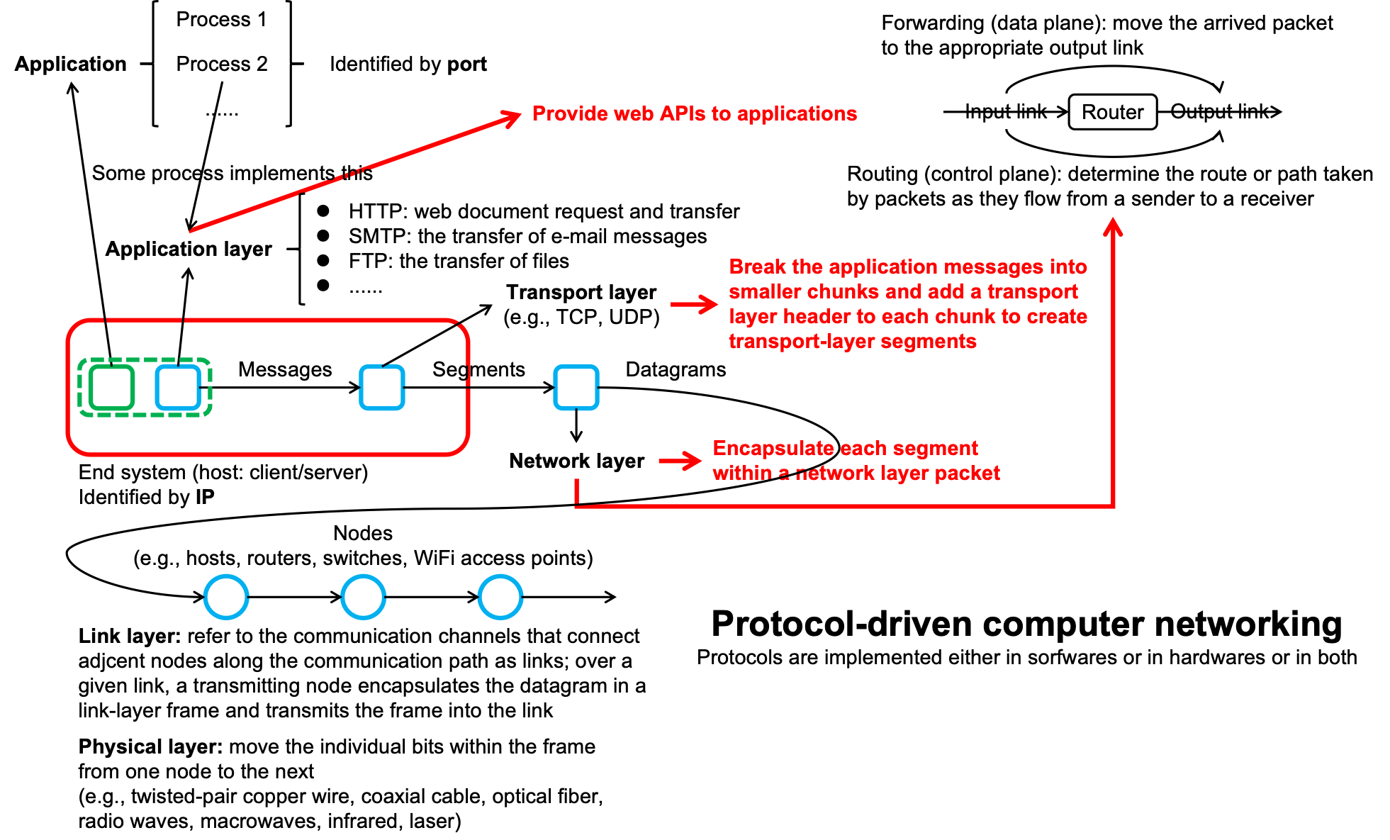

2.11.6 Working with networking

Click to see a larger version of the image — A rough scheme of five network layers

2.11.6.1 TCP (Transmission Control Protocol)

In a word, TCP provides highly reliable data transmission services with these features: connection-oriented, reliable, flow control, congestion control, error checking, slower than UDP due to providing such features.

using Sockets

## server side
errormonitor(@async begin
        server = listen(2000)  # 1. listen on a given port on a specified address; create a server waiting for incoming connections on the specified port 2000 in this case; a TCPServer socket is returned; in computer networking, a socket is a software structure that provides a bidirectional communication channel between two processes, where one process acts as a server and the other as a client
        while true
            sock = accept(server)  # 2. retrieve a connection to the client that is trying to connect to the server we just created
            @async while isopen(sock)  # 3. if connected, do something between the server and the client
                write(sock, string("The server has received the message from the client: ", readline(sock, keep = true)))  # 4. read something from the client and then write something to the client; keep = true means that these trailing newline characters are also returned (instead of removing them from the line before it is returned) as part of the line
            end
        end
end)

## client side
client = connect(2000)  # 1. connect to a host on a given port; return a TCPSocket socket

errormonitor(@async while isopen(client)  # 2. if connected, do something
    write(stdout, readline(client, keep = true))  # 3. read something from the server and then print them to the termimal (stdout)
end)

println(client, "Hello world from the client")  # 3. write something to the server
# The server has received the message from the client: Hello world from the client

## finally, use close() to disconnect the socket
close(client)

Note: some details about listen() and connect():

## 1. connect([host], port::Integer) -> TCPSocket  #  Connect to the host `host` on port `port` (TCPServer)
listen(2000)  # listen on localhost:2000 (IPv4)
listen(ip"127.0.0.1", 2000)  # equivalent to the above (IPv4)
listen(ip"::1", 2000)  # equivalent to the above (IPv6)
listen(IPv4(0), 2000)  # listen on port 2000 on all IPv4 interfaces
listen(IPv6(0), 2000)  # listen on port 2000 on all IPv6 interfaces

## 2. connect(path::AbstractString) -> PipeEndpoint  # connect to the named pipe (Windows) / UNIX domain socket at `path` (PipeServer)
listen("testsocket")  # listen on a UNIX domain socket
listen("\\\\.\\pipe\\testsocket")  # listen on a Windows named pipe (\\.\pipe\)

The difference between TCP and named pipes or UNIX domain sockets is subtle and has to do with the accept() and connect() methods:

accept(server[, client])  # Accepts a connection on the given server and returns a connection to the client. An uninitialized client stream may be provided, in which case it will be used instead of creating a new stream.

connect([host], port::Integer) -> TCPSocket  # Connect to the host `host` on port `port`.
connect(path::AbstractString) -> PipeEndpoint  # Connect to the named pipe / UNIX domain socket at path.

Resolving IP addresses:

julia> getaddrinfo("google.com")
# ip"59.24.3.174"

2.11.6.2 UDP (User Datagram Protocol)

UDP provides no such features as provided by TCP.

A common use for UDP is in multicast applications.

## receiver
using Sockets

group = ip"226.6.8.8"  # Choose a valid IP address for multicast: for IPv4, the multicast address range is from 224.0.0.0 to 239.255.255.255. Any address within this range is designated for multicast use. For IPv6, the multicast range begins with ff, such as ff05::5:6:7.
socket = UDPSocket()  # Open a UDP socket.
bind(socket, ip"0.0.0.0", 6688)  # Bind socket to the given host:port. Note that 0.0.0.0 (IPv4) / :: (IPv6) will listen on all devices (listen on all available network interfaces and all IPv4 / IPv6 addresses associated with the host machine. When binding to a port, make sure that the port number is not in use by another application and that it's not a well-known or registered port that has a specific protocol associated with it.
join_multicast_group(socket, group)  # Join a socket to a particular multicast group.
println(String(recv(socket)))  # For recv():  read a UDP packet from the specified socket, and return the bytes received. This call blocks.
# Hello over IPv4
leave_multicast_group(socket, group)  #  Remove a socket from a particular multicast group.
close(socket)  # Close the socket.

## sender
using Sockets

group = ip"226.6.8.8"
socket = UDPSocket()
send(socket, group, 6688, "Hello over IPv4")  #  Send msg over socket to host:port. It is not necessary for a sender to join the multicast group.
close(socket)

2.12 Parametric types

You can think of the expression S=P{T} as parametric type P taking a type parameter T and returning a new concrete type S. Both T and S are concrete types, while P is just a template for making types.

2.12.1 Defining parametric methods

function linearsearch(haystack::AbstractVector{T}, needle::T) where T
    for (i, x) in enumerate(haystack)
        if needle == x
            return i
        end
    end
end

linearsearch([1, 4, 6, 8], 6)

linearsearch([1, 4, 6, 8], "six")

MethodError: no method matching linearsearch(::Vector{Int64}, ::String)

Closest candidates are:
  linearsearch(::AbstractVector{T}, ::T) where T
   @ Main In[229]:1


Stacktrace:
 [1] top-level scope
   @ In[230]:2

In this example, the linearsearch() is a parametric method, which takes a type parameter T, defined in the where T clause. You can define more than one type parameter in the where clause (e.g. where {T, S}).

2.12.2 Defining parametric types

"A point at coordinate (x, y)"
struct Point{T}
    x::T
    y::T
end

Point

You can impose constraints on the type parameter T with subtype operator <::

struct RPoint{T<:Number}
    x::T
    y::T
end

When creating a point with Point, you can let Julia to infer the type parameter from arguments or explicitly set the type parameter:

Point(1, 2), Point{Int}(3, 4)

(Point{Int64}(1, 2), Point{Int64}(3, 4))

In fact, sum(xs::Vector) is the same as sum(xs::Vector{T}) where T.

In summary, parametric types can improve the type safety (stricter type checking), performance (more type restrictions, less type-related jobs), and memory usage (more type restrictions, more precise assignment of memory).

2.13 Scope of variables

2.13.1 Introduction

The scope of a variable is the region of code within which a variable is accessible. Variable scoping helps avoid variable naming conflicts.

There are two main types of scopes in programming languages: lexical scope (also called static scope) and dynamic scope.

In languages with lexical scope, the name resolution depends on the location in the source code and the lexical context, where the named variable is defined. In contrast, in languages with dynamic scope, the name resolution depends on the program state and the runtime context when the name is encountered.

In a word, with lexical scope a name is resolved by searching the local lexical context, then if that fails, by searching the outer lexical context, and so on; with dynamic scope, a name is resolved by searching the local execution context, then if that fails, by searching the outer execution context, and so on, progressing up the call stack.

Julia uses lexical scope. Further, there are two main types of scopes in Julia, global scope and local scope. The latter can be nested.

In Julia, different constructs may introduce different types of scopes.

2.13.2 Scope constructs

The constructs introducing scopes are:

Construct	Scope type	Allowed within
module, baremodule	global	global
struct	soft local	global
for, while, try	soft local	global, local
macro	hard local	global
functions, do blocks, let blocks, comprehensions, generators	hard local	global, local

Note: begin blocks and if blocks do not introduce scopes.

2.13.3 Global scope

Each module introduces a global scope.

Modules can introduce variables of other modules into their scopes through the using or import statement, or through qualified access using the dot notation.

module A
    a = 1  # a is a global variable in A's scope
end

module B
    module C
        c = 2
    end
    b = C.c  # can access the namespace of a nested global scope through a qualified access

    import ..A  # makes module A available
    d = A.a
end

If a top-level expression (e.g. a begin or if block) contains a variable declared with keyword local, then that variable is not accessible outside that expression.

x = 1
begin
    local x = 0
    @show x
end
@show x

x = 0
x = 1

Note: the REPL is in the global scope of the module Main.

2.13.4 Local scope

A local scope nested inside another local/global scope can see variables in all the outer scopes in which it is contained. Outer scopes, on the other hand, cannot see variables in inner scopes.

When x = <value> occurs in a local scope, Julia will apply the following rules to decide what the expression means:

Existing local: if x is already a local variable, then the existing local x is assigned.
Hard scope: if x is not already a local variable and this assignment occurs inside of any hard scope construct, then a new local variable named x is created in the scope of the assignment.
Soft scope: if x is not already a local variable and all of the scope constructs containing the assignment are soft scopes, the behavior depends on whether the global variable x is defined:
- If global x is undefined, a new local variable named x is created in the scope of the assignment;
- If global x is defined, then the following rules are applied:
  - In interactive mode, the global variable x is assigned;
  - In non-interactive mode, an ambiguity warning is printed and a new local variable named x is created in the scope of the assignment.

Therefore, in non-interactive mode, the soft scope and hard scope behaves identically except that a warning is printed when an implicitly local variable shadows a global variable in the soft scope.

Note: in Julia, a variable cannot be a non-local variable, meaning that it is either a local variable or a global variable, which is determined regardless of the order of expressions. As a consequence, if you assign to an existing local, it always updates that existing local; therefore, you can only shadow a local by explicitly declaring a new local in a nested scope with the local keyword.

function outer_foo()
    x = 99  # x is a local variable in the outer_foo's scope
    @show x
    let
        x = 100  # updates the local variable x defined in the outer_foo's scope
    end
    @show x
    return nothing
end

outer_foo (generic function with 1 method)

code = """
s = 0 # global
for i = 1:10
    t = s + i # new local t
    s = t # new local s with warning
end
s # global; should be 0
@isdefined(t) # t is local, not global; should be false
"""

include_string(Main, code)

LoadError: LoadError: UndefVarError: `s` not defined
in expression starting at string:2
LoadError: UndefVarError: `s` not defined
in expression starting at string:2

Stacktrace:
 [1] top-level scope
   @ ./string:3
 [2] eval
   @ ./boot.jl:385 [inlined]
 [3] include_string(mapexpr::typeof(identity), mod::Module, code::String, filename::String)
   @ Base ./loading.jl:2139
 [4] include_string
   @ ./loading.jl:2149 [inlined]
 [5] include_string(m::Module, txt::String)
   @ Base ./loading.jl:2149
 [6] top-level scope
   @ In[236]:12

Caution

So don’t forget to use the global keyword to declare a variable x if you want to use a global x instead of a local x in seeing a for loop in non-interactive mode:

code = """
s = 0
for i in 1:100
    global s = s + i
end
@show s
"""

include_string(Main, code)

s = 5050

2.13.5 `let` blocks

let blocks create a new hard local scope and introduce new variable bindings each time they run. The variable need not be immediately assigned. The value evaluated from the last expression is returned.

let x  # x need not be immediately assigned
    x = 1
end

The let syntax accepts a comma-separated series of assignments and variable names.

x, y = 1, 2

let x = x, y = 20
    @show x, y
end

(x, y) = (1, 20)

(1, 20)

Note: in the above example, x = x is possible, since the assignment is evaluated from the right to the left. x in the right-hand side is global; x in the left-hand side is local.

2.13.6 Loops

A for loop iteration variable is always a new local variable; otherwise you declare it using the outer keyword.

function for_f1()
    i = 0
    for i = 1:3  # i is local
    end
    return i
end

for_f1()

function for_f2()
    i = 0
    for outer i = 1:3  # i is global
    end
    return i
end

for_f2()

A noteworthy fact is that you must declare i using the global keyword in the following code or an error will be raised when you run it in non-interactive mode:

code = """
    i = 10
    while i <= 12
        i = i + 1  # i is regarded as a local instead of a global since this is determined regardless of the order of expressions
        @show i
    end
    @show i
"""

include_string(Main, code)

LoadError: LoadError: UndefVarError: `i` not defined
in expression starting at string:2
LoadError: UndefVarError: `i` not defined
in expression starting at string:2

Stacktrace:
 [1] top-level scope
   @ ./string:3
 [2] eval
   @ ./boot.jl:385 [inlined]
 [3] include_string(mapexpr::typeof(identity), mod::Module, code::String, filename::String)
   @ Base ./loading.jl:2139
 [4] include_string
   @ ./loading.jl:2149 [inlined]
 [5] include_string(m::Module, txt::String)
   @ Base ./loading.jl:2149
 [6] top-level scope
   @ In[242]:11

code = """
    i = 10
    while i <= 12
        global i = i + 1  # i is global
        @show i
    end
    @show i
"""

include_string(Main, code)

i = 11
i = 12
i = 13
i = 13

2.13.7 Constants

The const declaration should only be used in global scope on globals. It is difficult for the compiler to optimize code involving global variables, since their values (or even their types) might change at almost any time. If a global variable will not change, adding a const declaration solves this performance problem.

Local constants are quite different. The compiler is able to determine automatically when a local variable is constant, so local constant declarations are not necessary, and in fact are currently not supported.

2.13.8 Typed globals

A global can be declared to always be of a constant type by using the syntax global x::T or upon assignment as x::T = 123.

Once a global is declared to be of a constant type, it cannot be assigned to values which cannot be converted to the specified type. In addition, a global has either been assigned to or its type has been set, the binding type is not allowed to change.

2.14 Parallel computing

2.14.1 Asynchronous tasks

A task has a create-start-run-finish lifecycle, allowing suspending and resuming computations.

Create a task by calling the Task constructor on a 0-argument function or using the @task macro: Task(() -> x) is equivalent to @task x.
Start a task by calling schedule(x) (i.e., add it to an internal queue of tasks).

Note: for convenience, you can use @async x to create and start a task at once (equivalent to schedule(@task x)).

You can then call wait(x) to wait the task to exit.

function mysleep(seconds)
    sleep(seconds)
    println("done")
end

t = Task(() -> mysleep(5))  # equivalent to `@task mysleep(5)`
schedule(t)
wait(t)

done

Communicating with channels.

You can call the Channel{T}(size) constructor to create a channel with an internal buffer that can hold a maximum of size objects of type T (Channel(0) constructs an unbuffered channel).
Different tasks can write to the same channel concurrently via put!(channel, x) calls.
Different tasks can read data concurrently via take!(channel) (remove and return a value from a channel) or fetch() (return the first available value from a channel without removing) calls.
If a channel is empty, readers (on a take!() call) will block until data is available.
If a channel is full, writers (on a put!() call) will block until space becomes available.
You can use isready(channel) to check for the presence of any object in the channel, and use wait(channel) to wait for an object to become available.
You can use close(channel) to close a channel. On a closed channel, put!() will fail, but take!() and fetch() can still successfully return any existing values until it is emptied.
You can associate a channel with a task using the Channel(f) constructor (f is a function accepting a single argument of type Channel) or the bind(channel, task) function. This means that the lifecycle of the channel is bound to this task (i.e., you don’t have to close the channel explicitly, while the channel will be closed the moment the task exits). In addition, it will not only log any unexpected failures, but also force the associated resources to close and propagate the exception everywhere. Compared with bind(), errormonitor(task) only prints an error log if task fails.
The returned channel can be used as an iterable object in a for loop, in which case the loop variable takes on all the produced values. The loop is terminated when the channel is closed.

jobs = Channel{Int}(32)
results = Channel{Tuple}(32)

function do_work()
    for job_id in jobs
        exec_time = rand()
        sleep(exec_time)

        put!(results, (job_id, exec_time))
    end
end

function make_jobs(n)
    for i in 1:n
        put!(jobs, i)
    end
end

n = 12

errormonitor(@async make_jobs(n))

for i in 1:4  # spawn 4 tasks
    errormonitor(@async do_work())
end

sum_time = 0
eval_time = @elapsed while n > 0
    job_id, exec_time = take!(results)
    println("$job_id finished in $(round(exec_time; digits = 2)) seconds")
    global n = n - 1
    global sum_time = sum_time + exec_time
end
println("The evaluated time is $eval_time seconds")
println("The accumulated time is $sum_time seconds")

2 finished in 0.07 seconds
4 finished in 0.32 seconds
1 finished in 0.44 seconds
3 finished in 0.53 seconds
8 finished in 0.01 seconds
5 finished in 0.56 seconds
6 finished in 0.44 seconds
9 finished in 0.28 seconds
12 finished in 0.03 seconds
7 finished in 0.56 seconds
11 finished in 0.77 seconds
10 finished in 0.93 seconds
The evaluated time is 1.784854254 seconds
The accumulated time is 4.927229826696577 seconds

More task operations

Task operations are built on a low-level primitive called yieldto(task, value), which suspends the current task, switches to the specified task, and causes that task’s last yieldto() call to return the specified value.

A few other useful functions of tasks:

current_task(): gets a reference to the currently-running task.
istaskdone(): queries whether a task has exited.
istaskstarted(): queries whether a task has run yet.
task_local_storage(): manipulates a key-value store specific to the current task.

2.14.2 Multi-threading

Julia’s multi-threading, provided by the Threads module, a sub-module of Base, provides the ability to schedule tasks simultaneously on more than one thread or CPU core, sharing memory.

2.14.2.1 Starting Julia with multiple threads

The number of execution threads is controlled either by using -t/--threads (julia -t 4) command line argument or by using the JULIA_NUM_THREADS (export JULIA_NUM_THREADS=4, which must be done before starting Julia, and setting it in startup.jl file by using ENV is too late) environment variable. When both are specified, the -t/--threads takes precedence. Both options support the auto argument, which let Julia itself infer a useful default number of threads to use.

Note: The number of threads specified with -t/--threads is propagated to processes that are spawned using the -p/--procs or --machine-file command line option. For example, julia -p 2 -t 2 spawns 1 main process and 2 worker processes, and all three processes have 2 threads enabled. For more fine grained control over worker threads use addprocs() and pass -t/--threads as exeflags.

Note: The Garbage Collector (GC) can use multiple threads. You can specify it either by using the --gcthreads command line argument or by using the JULIA_NUM_GC_THREADS environment variable.

After starting Julia with multiple threads, you can check it with the following functions:

Threads.nthreads()

Threads.threadid()

2.14.2.2 Thread pools

There are two types of thread pools: :interactive (often used for interactive tasks) and :default (often used for long duration tasks).

You can set the number of execution threads available for each thread pool of the two by: -t 3,1 or JULIA_NUM_THREADS=3,1, which means that there are 3 threads in the :default thread pool, and 1 thread in the :interactive thread pool. Both numbers can be replaced with the word auto.

Corresponding helper functions:

using Base.Threads

println(nthreadpools())  # the number of thread pools

println(threadpool(1))  # which thread pool the thread 1 belongs to

println(nthreads(:default))  # the number of threads available for the :default thread pool

2
default
1

2.14.2.3 Spawning threads

@spawn: you can specify which thread pool should be used by the spawned thread.

Threads.@spawn :interactive begin; println("task done"); end

task done

Task (done) @0x0000724ffe13f530

@threads: this macro is affixed in front of a for loop to indicate to Julia that the loop is a multi-threaded region.

a = zeros(10)

# the iteration space is plit among the threads
Threads.@threads for i = 1:10
    a[i] = Threads.threadid()
end

a

10-element Vector{Float64}:
 1.0
 1.0
 1.0
 1.0
 1.0
 1.0
 1.0
 1.0
 1.0
 1.0

Note: after a task starts running on a certain thread it may move to a different thread although the :static schedule option for @threads does freeze the thread id. This means that in most cases threadid() should not be treated as constant within a task.

2.14.2.4 Avoiding data race

Be very careful about reading any data if another thread might write to it!

Instead, always use the lock pattern when changing data accessed by other threads.

lk = ReentrantLock()

# method 1
lock(lk) do 
    use(a)
end

# method 2
begin
    lock(lk)
    try
        use(a)
    finally
        unlock(lk)  # each lock must be matched by an unlock
    end
end

A toy example:

Without multi-threading:

# the correct result
function sum_single(x)
    s = 0
    for i = x
        s += i
    end
    s
end

@time sum_single(1:1_000_000)  # in Julia, the underscore (_) can be used as a separator in literal integers to enhance readability

  0.000001 seconds

500000500000

Data race often leads to non-deterministic results:

# with data race and the result is non-deterministic
function sum_multi_bad(x)
    s = 0
    Threads.@threads for i = x
        s += i
    end
    s
end

for i = 1:6
    println(sum_multi_bad(1:1_000_000))
end

500000500000
500000500000
500000500000
500000500000
500000500000
500000500000

Add lock when performing data race operations:

# locked version
# the result is correct
lk = ReentrantLock()

function sum_multi_lock(x)
    s = 0
    Threads.@threads for i = x
        lock(lk) do
            s += i
        end
    end
    s
end

for i = 1:6
    println(sum_multi_lock(1:1_000_000))
end

500000500000
500000500000
500000500000
500000500000
500000500000
500000500000

Split data into chunks –> use its own internal buffer for each thread –> collect all results of chunks:

# split the sum into chunks that are race-free
# collect the result of each chunk
# add the results together
function sum_multi_chunk(x)
    chunks = Iterators.partition(x, length(x) ÷ Threads.nthreads())
    tasks = map(chunks) do chunk
        Threads.@spawn sum_single(chunk)
    end
    chunk_sums = fetch.(tasks)
    return sum_single(chunk_sums)
end

@time sum_multi_chunk(1:1_000_000)

  0.047882 seconds (15.59 k allocations: 1.082 MiB, 99.68% compilation time)

500000500000

Use atomic operations:

Julia supports accessing and modifying values atomically, that is, in a thread-safe way to avoid data race.

A value (which must be of a primitive type) can be wrapped as Threads.Atomic{T}(value) to indicate it must be accessed in this way.

In a word, perform atomic operations on atomic values to avoid data race.

function sum_multi_atomic(x)
    s = Threads.Atomic{Int}(0)  # s is an atomic value of type Int
    Threads.@threads for i = x
        Threads.atomic_add!(s, i)  # perform atomic operation atomic_add! (add i to s, and return the old value) on atomic value s
    end
    s
end

res = sum_multi_atomic(1:1_000_000)
res[]  # Atomic objects can be accessed using the [] notation

500000500000

2.14.3 Multi-processing and Distributed computing

Distributed computing provided by module Distributed runs multiple Julia processes with separate memory spaces.

2.14.3.1 Starting and managing multiple processes

In Julia, each process has an associated identifier. The process providing the interactive Julia prompt always has an id equal to 1, called the main process.

By default, the processes used for parallel operations are referred to as “workers”. When there is only 1 process, process 1 is considered a worker. Otherwise, workers are considered to be all processes other than process 1. As a result, adding 2 or more processes is required to gain benefits from parallel processing methods. Adding a single process is beneficial if you just wish to do other things in the main process while a long computation is running on the worker.

Julia has built-in support for two types of clusters:

A local cluster specified with the -p/--procs option (implicitly loads module Distributed).
A cluster spanning machines using the --machine-file option.

This uses a passwordless ssh login to start Julia worker processes from the same path as the current host on the specified machines.

Each machine definition takes the form [count*] [user@]host[:port] [bind_addr[:port]]. count is the number of workers to spawn on the node, and defaults to 1; user defaults to the current user; port defaults to the standard ssh port; bind_addr[:port] specifies the IP address and port that other workers should use to connect to this worker.

Note: in Julia, distribution of code to worker processes relies on Serialization.serialize (the need for data serialization and deserialization arises primarily due to the requirement to convert complex data structures into formats that can be transmitted across a network when different nodes communicate with each other), so it is advised that all workers on all machines use the same version of Julia to ensure compatibility of serialization and deserialization.

Distributed package provides some useful functions for starting and managing processes within Julia:

using Distributed  # Module Distributed must be explicitly loaded on the master process before invoking addprocs() and other functions if you want to start distributed computing within Julia, instead of using command line options. It is automaticaly made available on the worker processes.

addprocs()  # launch worker processes using the LocalManager (the same as -p), SSHManager (the same as --machine-file) or other cluster managers of type ClusterManager

procs()  # return a list of all process identifiers

nprocs()  # return the number of available processes

workers()

nworkers()

myid()  # get the id of the current process

Note: workers do not run a ~/.julia/config/startup.jl startup script, nor do they synchronize their global state with any of the other running processes. You may use addprocs(exeflags = "--project") to initialize a worker with a particular environment.

Network requirements for LocalManager and SSHManager

The master process does not listen on any port. It only connects out to the workers.
Each worker binds to only one of the local interfaces and listens on an ephemeral port number assigned by the OS.
LocalManager, used by addprocs(N), by default binds only to the loopback interface. An addprocs(4) followed by an addprocs(["remote_host"]) will fail. To create a cluster comprising their local system and a few remote systems, it can be done by explicitly requesting LocalManager to bind to an external network interface via restrict keyword argument: addprocs(4; restrict = false).
SSHManager, used by addprocs(list_of_remote_hosts), launches workers on remote hosts via SSH. By default SSH is only used to launch Julia workers. Subsequent master-worker and worker-worker connections use plain, unencrypted TCP/IP sockets. The remote hosts must have passwordless login enabled. Additional SSH flags or credentials may be specified via keyword argument sshflags.

Cluster cookie

All processes in a cluster share the same cookie which, by default, is a randomly generated string on the master process, and can be accessed via cluster_cookie(), while cluster_cookie(cookie) sets it and returns the new cookie. It can also be passed to the workers at startup via --worker=<cookie>.

Specifying network topology

The keyword argument topology to addprocs() is used to specify how the workers must be connected to each other. The default is :all_to_all, meaning that all workers are connected to each other.

2.14.3.2 Starting distributed programming

Distributed programming in Julia is built on two primitives:

Remote references: a remote reference is an object of type RemoteChannel that can be used from any process to refer to an object stored on a particular process. Multiple processes can communicate via RemoteChannel.
Remote calls: a remote call is a request by one process to call a certain function on certain arguments on another (possibly the same) process. A remote call returns a Future object to its result. Then you can use wait() to wait the function running to finish or use fetch() to get the returned value by the called function.

Launch remote calls:

@spawn p expr  # Create a closure around an expression and run the closure asynchronously on process p. If p is set to :any, then the system will pick a process to use automatically.
@fetchfrom p expr  # equivalent to fetch(@spawnat p expr)

remotecall(f, pid, ...)  # Call a function f asynchronously on the given arguments ... on the specified process pid.
remotecall(f, pool, ...)  # Give a pool of type WorkerPool instead of a pid. It will wait for and take a free worker from pool to use.
remotecall_fetch()  # equivalent to fetch(remotecall())
remote_do(f, id, ...)  # Run f on worker id asynchronously. Unlike remotecall, it does not store the result of computation, nor is there a way to wait for its completion.

using Distributed

addprocs(2)  # add 2 wrokers via LocalManager

r = remotecall(rand, 2, 3, 3)  # run rand(3, 3) on process 2
s = @spawnat 2 1 .+ fetch(r)  # run expr 1 .+ fetch(r) on process 2 (note: this forms a closure () -> 1 .+ fetch(r) which contains the global variable r)
fetch(s)

3×3 Matrix{Float64}:
 1.04629  1.54029  1.15181
 1.74728  1.54821  1.7228
 1.59677  1.8041   1.40291

Note: once fetched, a Future will cache its value locally. Further fetch() calls don not entail a network hop. Once all referencing Futures have fetched, the remote stored value is deleted.

2.14.3.3 Code and data availability

Before spawning a process, you must ensure that your code and data are available on any process that runs it.

Code availability

function rand2(dims...)
    return 2 * rand(dims...)
end

rand2(2, 2)

2×2 Matrix{Float64}:
 0.0602265  1.47168
 0.0996057  0.625218

using Distributed

addprocs(2)

# rand2 is defined in the main process
# so process 1 knew it but the others did not
fetch(@spawnat :any rand2(2, 2))

On worker 2:
UndefVarError: `#rand2` not defined
Stacktrace:
  [1] deserialize_datatype
    @ /data/softwares/julia_v1.10.7/share/julia/stdlib/v1.10/Serialization/src/Serialization.jl:1399
  [2] handle_deserialize
    @ /data/softwares/julia_v1.10.7/share/julia/stdlib/v1.10/Serialization/src/Serialization.jl:867
  [3] deserialize
    @ /data/softwares/julia_v1.10.7/share/julia/stdlib/v1.10/Serialization/src/Serialization.jl:814
  [4] handle_deserialize
    @ /data/softwares/julia_v1.10.7/share/julia/stdlib/v1.10/Serialization/src/Serialization.jl:874
  [5] deserialize
    @ /data/softwares/julia_v1.10.7/share/julia/stdlib/v1.10/Serialization/src/Serialization.jl:814 [inlined]
  [6] deserialize_global_from_main
    @ /data/softwares/julia_v1.10.7/share/julia/stdlib/v1.10/Distributed/src/clusterserialize.jl:160
  [7] #5
    @ /data/softwares/julia_v1.10.7/share/julia/stdlib/v1.10/Distributed/src/clusterserialize.jl:72 [inlined]
  [8] foreach
    @ ./abstractarray.jl:3098
  [9] deserialize
    @ /data/softwares/julia_v1.10.7/share/julia/stdlib/v1.10/Distributed/src/clusterserialize.jl:72
 [10] handle_deserialize
    @ /data/softwares/julia_v1.10.7/share/julia/stdlib/v1.10/Serialization/src/Serialization.jl:960
 [11] deserialize
    @ /data/softwares/julia_v1.10.7/share/julia/stdlib/v1.10/Serialization/src/Serialization.jl:814
 [12] handle_deserialize
    @ /data/softwares/julia_v1.10.7/share/julia/stdlib/v1.10/Serialization/src/Serialization.jl:871
 [13] deserialize
    @ /data/softwares/julia_v1.10.7/share/julia/stdlib/v1.10/Serialization/src/Serialization.jl:814
 [14] handle_deserialize
    @ /data/softwares/julia_v1.10.7/share/julia/stdlib/v1.10/Serialization/src/Serialization.jl:874
 [15] deserialize
    @ /data/softwares/julia_v1.10.7/share/julia/stdlib/v1.10/Serialization/src/Serialization.jl:814 [inlined]
 [16] deserialize_msg
    @ /data/softwares/julia_v1.10.7/share/julia/stdlib/v1.10/Distributed/src/messages.jl:87
 [17] #invokelatest#2
    @ ./essentials.jl:892 [inlined]
 [18] invokelatest
    @ ./essentials.jl:889 [inlined]
 [19] message_handler_loop
    @ /data/softwares/julia_v1.10.7/share/julia/stdlib/v1.10/Distributed/src/process_messages.jl:176
 [20] process_tcp_streams
    @ /data/softwares/julia_v1.10.7/share/julia/stdlib/v1.10/Distributed/src/process_messages.jl:133
 [21] #103
    @ /data/softwares/julia_v1.10.7/share/julia/stdlib/v1.10/Distributed/src/process_messages.jl:121

Stacktrace:
 [1] remotecall_fetch(f::Function, w::Distributed.Worker, args::Distributed.RRID; kwargs::@Kwargs{})
   @ Distributed /data/softwares/julia_v1.10.7/share/julia/stdlib/v1.10/Distributed/src/remotecall.jl:465
 [2] remotecall_fetch(f::Function, w::Distributed.Worker, args::Distributed.RRID)
   @ Distributed /data/softwares/julia_v1.10.7/share/julia/stdlib/v1.10/Distributed/src/remotecall.jl:454
 [3] remotecall_fetch
   @ /data/softwares/julia_v1.10.7/share/julia/stdlib/v1.10/Distributed/src/remotecall.jl:492 [inlined]
 [4] call_on_owner
   @ /data/softwares/julia_v1.10.7/share/julia/stdlib/v1.10/Distributed/src/remotecall.jl:565 [inlined]
 [5] fetch(r::Future)
   @ Distributed /data/softwares/julia_v1.10.7/share/julia/stdlib/v1.10/Distributed/src/remotecall.jl:619
 [6] top-level scope
   @ /data/softwares/julia_v1.10.7/share/julia/stdlib/v1.10/Distributed/src/macros.jl:95

Note: more commonly you’ll be loading code from files or packages, and you’ll have a considerable amount of flexibility in controlling which processes load code. So if you have defined some functions, types, etc., you’d better organize them into files or packages, which will make things easier.

Consider a file, DummyModule.jl, containing the following code:

module DummyModule
export MyType, f

mutable struct MyType
    a::Int
end

f(x) = x^2 + 1

println("DummyModule loaded")

end

In order to refer to the code defined in DummyModule.jl across all processes, first, DummyModule.jl needs to be loaded on every process. Calling include("DummyModule.jl") loads it only on a single process. To load it on every process, use the @everywhere [procs()] expr macro, which execute an expression under Main on all procs:

@everywhere include("DummyModule.jl")
@everywhere using InteractiveUtils

@fetchfrom 2 InteractiveUtils.varinfo()  # show exported global variables in a module

DummyModule loaded
      From worker 2:    DummyModule loaded
      From worker 3:    DummyModule loaded

name	size	summary
Base		Module
Core		Module
Distributed	1.131 MiB	Module
DummyModule	266.805 KiB	Module
Main		Module
r	256 bytes	Future

Once loaded, we can use code defined in DummyModule.jl across all processes by:

@everywhere using .DummyModule

@fetchfrom 2 f(100)

      From worker 2:    ┌ Warning: Cannot transfer global variable f; it already has a value.
      From worker 2:    └ @ Distributed /data/softwares/julia_v1.10.7/share/julia/stdlib/v1.10/Distributed/src/clusterserialize.jl:166

Note: a file can be preloaded on multiple processes at startup with the -L flag, and a driver script can be used to drive the computation: julia -p <n> -L file1.jl -L file2.jl driver.jl. The Julia process running the driver script given here has an id equal to 1, just like a process providing an interactive prompt.

If DummyModule.jl is a package, just use @everywhere using DummyModule, which will make code defined in DummyModule.jl available in every process.

Data availability

Sending messages and moving data constitute most of the overhead in a distributed program.

Reducing the number of messages and the amount of data sent is critical to achieving performance and scalability.

Global variables

Expressions executed remotely via @spawnat, or closures specified for remote execution using remotecall() may refer to global variables.

Remote calls with embedded global references (under Main module only) manage globals as follows:
- New global bindings are created on destination workers if they are referenced as part of remote call.
- Global constants are declared as constants on remote nodes too.
- Globals are re-sent to a destination worker only in the context of a remote call, and only if its value has changed.
- The cluster does not synchronize global bindings across nodes.

Note: memory associated with globals may be collected when they are reassigned on the master, while no such action is taken on the workers as the bindings continue to be valid. clear!() can be used to manually reassign specific globals on remote nodes to nothing once they are no longer required.

Only when remote calls refer to globals under the Main module are new global bindings created on destination workers, so we can use let blocks to localize global variables when forming closures. This avoids new global bindings’ creating on destination workers:

A = rand(10, 10)
remotecall_fetch(() -> A, 2)  # A is a global variable under the Main module, so new global binding of A will be created on process 2

B = rand(10, 10)
let B = B  # B becomes a local variable, so B won't be created on process 2
    remotecall_fetch(() -> B, 2)
end
@fetchfrom 2 InteractiveUtils.varinfo()

name	size	summary
A	840 bytes	10×10 Matrix{Float64}
Base		Module
Core		Module
Distributed	1.138 MiB	Module
DummyModule	267.636 KiB	Module
Main		Module
r	256 bytes	Future

Communicating with RemoteChannels

Create references to remote channels with the following:
```
RemoteChannel(f, pid)  # Create references to remote channels of a specific size and type. f is a function that when executed on pid (the default is the current process) must return an implementation of an AbstractChannel. e.g., RemoteChannel(() -> Channel{Int}(10), pid).
RemoteChannel(pid)  # make a reference to a Channel{Any}(1) on process pid
```
- A Channel is local to a process, but a RemoteChannel can put and take values across workers.
- A RemoteChannel can be thought of as a handle to a Channel.
- The process id, pid, associated with a RemoteChannel identifies the process where the backing store, i.e., the backing Channel exists.
- Any process with a reference to a RemoteChannel can put and take items from the channel. Data is automatically sent to or retrieved from the process a RemoteChannel is associated with.
- Serializing a Channel also serializes any data present in the channel. Deserializing it therefore effectively makes a copy of the original object.
- On the other hand, serializing a RemoteChannel only involves the serialization of an identifier that identifies the location and instance of Channel referred to by the handle. A deserialized RemoteChannel object on any worker, therefore also points to the same backing store as the original.

jobs = RemoteChannel(() -> Channel{Int}(32))
results = RemoteChannel(() -> Channel{Tuple}(32))

@everywhere function do_work(jobs, results)  # define work function everywhere
    while true
        job_id = take!(jobs)
        exec_time = rand()
        sleep(exec_time)  # simulate elpased time doing actual work
        put!(results, (job_id, exec_time, myid()))
    end
end

function make_jobs(n)
    for i in 1:n
        put!(jobs, i)
    end
end

n = 12

errormonitor(@async make_jobs(n))

for p in workers()
    remote_do(do_work, p, jobs, results)
end

@elapsed while n > 0
    job_id, exec_time, where = take!(results)
    println("$job_id finished in $(round(exec_time; digits = 2)) seconds on worker $where")
    global n = n - 1
end

1 finished in 0.5 seconds on worker 2
2 finished in 0.55 seconds on worker 3
4 finished in 0.23 seconds on worker 3
3 finished in 0.88 seconds on worker 2
6 finished in 0.04 seconds on worker 2
5 finished in 0.99 seconds on worker 3
8 finished in 0.3 seconds on worker 3
7 finished in 0.98 seconds on worker 2
10 finished in 0.33 seconds on worker 2
11 finished in 0.06 seconds on worker 2
9 finished in 0.84 seconds on worker 3
12 finished in 0.67 seconds on worker 2

4.118156453

Local invocations

When data is stored on a different node from the execution node, data is necessarily copied over to the remote node for execution. However, when the destination node is the local node, i.e., the calling process id is the same as the remote node id, it is executed as a local call. It is usually (not always) executed in a different task, but there is no serialization/deserialization of data. Consequently, the call refers to the same object instances as passed, i.e., no copies are created.

rc = RemoteChannel(() -> Channel(3))  # RemoteChannel created on local node

v = [0]  # array in Julia has stable memory address

for i in 1:3
    v[1] = i  # reusing v
    put!(rc, v)
end

res = [take!(rc) for _ in 1:3]

println(res)

println(map(objectid, res))

println("Num unique obejcts: ", length(unique(map(objectid, res))))

[[3], [3], [3]]
UInt64[0x8d26183d637b3471, 0x8d26183d637b3471, 0x8d26183d637b3471]
Num unique obejcts: 1

In general, this is not an issue. If the local node is also being used as a compute node, and the arguments used post the call, this behavior needs to be factored in and if required deep copies of arguments.

Shared arrays

Shared arrays use system shared memory to map the same array across many processes.

Each “participating” process has access to the entire array, which is totally different from the DArray defined in DistributedArrays.jl, of which each process has local access to just a chunk (i.e., no two processes share the same chunk).

A SharedArray defined in SharedArrays module is a good choice when you want to have a large amount of data jointly accessible to two or more processes on the same machine.

In cases where an algorithm insists on an Array input, the underlying array can be retrieved from a SharedArray by calling sdata(). For other AbstractArray types, sdata() just returns the object itself.

The constructor for a shared array is of the form: SharedArray{T, N}(dims::NTuple; init=false, pids=Int[]), by which we can construct an N-dimensional shared array of a bits type (check whether an element is supported using isbits()) T and size dims across the processes specified by pids. If an initialization function of the form f(S::SharedArray) is passed to init, then it is called on all the participating workers. You can specify that each worker runs the init function on a distinct portion of the array, thereby parallelizing initialization.

@everywhere using SharedArrays

S = SharedArray{Int, 2}((3, 4), init = S -> S[localindices(S)] = repeat([myid()], length(localindices(S))))

# localindices(S): return a range describing the "default" indices to be handled by the current process.
# indexpids(S): return the current worker's index (starting from 1, not the same as the actual pid) in the list of workers mapping the SharedArray, or 0 if the SharedArray is not mapped onto the current process.
# procs(S): return the list of pids mapping the SharedArray.

3×4 SharedMatrix{Int64}:
 2  2  3  3
 2  2  3  3
 2  2  3  3

Note: because any process mapping the SharedArray has access to the entire array, you must take consideration on possible operation conflicts.

2.14.3.4 Parallel loops and map

Looping and then reducing

Many iterations run independently over several processes, and then their results are combined using some function (the result of each iteration is taken as the value of the last expression inside the loop) . The combination process is called a reduction. In code, this typically looks like the pattern x = f(x, v[i]), where x is the accumulator, f is the reduction function, and v[i] are the elements being reduced. It is desirable for f to be associative, so that it does not matter what order the operations are performed in.

# When reducer is given, it will be blocked and return the final result of reduction process.
# @distributed [reducer] for var = range
#     body
# end

# reducer is optional.
# If it is omitted, then it will return a Task object immediately without waiting for completion.
# You can prefix @sync or add wait(t) or fetch(t) (returns nothing) after it to wait for completion.
 # @sync @distributed for var = range
 #    body
 # end

res = @distributed (vcat) for i in 1:6
    [(myid(), i)]
end

res

6-element Vector{Tuple{Int64, Int64}}:
 (2, 1)
 (2, 2)
 (2, 3)
 (3, 4)
 (3, 5)
 (3, 6)

Mapping

If we merely want to apply a function to all elements in some collection, we can use parallelized map, implemented in Julia as the pmap() function.

using LinearAlgebra

M = Matrix{Float64}[rand(1000, 1000) for _ in 1:10]
pmap(svdvals, M)  # calculate the singular values of several matrices in parallel

10-element Vector{Vector{Float64}}:
 [499.79679885693923, 18.38329981098877, 18.13504957827479, 18.03902647832188, 17.96266157226113, 17.900590664350776, 17.812632711106865, 17.799135095257196, 17.75321377403185, 17.74884986706717  …  0.12862899278647885, 0.11607226057893819, 0.10311954532424052, 0.09877271936853954, 0.08290088194742752, 0.06955148590104983, 0.06456481667674498, 0.032973776992069596, 0.017414128706166567, 0.013848102591456921]
 [500.1505933307007, 18.286933282027977, 17.96778330579176, 17.94529885426076, 17.829526833127762, 17.812689508510235, 17.76419141512595, 17.673791231132704, 17.62014733202228, 17.56208421582004  …  0.13450823497726025, 0.11772522328505304, 0.10219613279239266, 0.08658559390518596, 0.08039026897383579, 0.06948594985302062, 0.0553534480406535, 0.043166090720678084, 0.009502109328058318, 0.007413419496910726]
 [499.93802718379703, 18.245481074658937, 18.0514265417282, 17.943708760345615, 17.905030146014088, 17.804173292686645, 17.772012655108295, 17.751207306106785, 17.63346722875819, 17.599410303197434  …  0.13511693414608025, 0.12159967933204514, 0.10009410734669874, 0.09733404504064472, 0.08261006744473588, 0.070327491499848, 0.05045521672240982, 0.03840940303990619, 0.0064086388406943496, 0.005197025112704688]
 [500.40906678017507, 18.237025238851405, 18.013198825052832, 17.966211160612072, 17.83209099323381, 17.80777431780662, 17.780512293878243, 17.728969870599297, 17.580919777114836, 17.559361855711224  …  0.12042348272501828, 0.11529749516204225, 0.09818914662643448, 0.08269033269987981, 0.0816520762137033, 0.06549884474462586, 0.05152637928791907, 0.04435613250853343, 0.024990747660403795, 0.002696146447039039]
 [500.58952277956024, 18.423303226931147, 18.06986920554837, 17.952305152969704, 17.839475751411058, 17.75518143094209, 17.69822183113631, 17.674718837951854, 17.64996453061288, 17.592963850562185  …  0.13063394689263116, 0.12430607157847853, 0.1074046746905318, 0.09787829202705449, 0.07888487107545679, 0.06809677099868564, 0.039349176047031136, 0.01974204840883153, 0.017222315150805873, 0.011454674834089577]
 [500.01996903853893, 18.126575962719198, 18.006454569319196, 17.888865984690757, 17.83860935944013, 17.807930780898257, 17.73671037230043, 17.669666940738804, 17.625192993586843, 17.546824477461655  …  0.14162053439522493, 0.12068588961919258, 0.11197702285816027, 0.09537142468173265, 0.08181013811345315, 0.06823646661904631, 0.051547105209096195, 0.037929278786833595, 0.02855215911727032, 0.0038092021005507017]
 [500.229097139824, 18.10453224943811, 18.049116482867777, 17.9573598088194, 17.84068641965531, 17.781706349897302, 17.75270763057804, 17.711268642271797, 17.625309566501432, 17.603413679631213  …  0.1323365287833669, 0.12639736237046642, 0.10162622107933063, 0.09581020413179003, 0.06731744608321613, 0.06226972026336506, 0.048646248399650545, 0.025756578952127584, 0.02024899813520592, 0.0034040075346289007]
 [500.20058569902585, 18.192042248403684, 18.078275009964234, 17.982007255329577, 17.92739711691456, 17.87235247229389, 17.819495274752075, 17.692493419176348, 17.63615562987625, 17.583716375112722  …  0.13391636025549528, 0.11915389682631942, 0.11551510123552947, 0.09031339497022907, 0.0790008363928607, 0.07082893292790585, 0.04658844538729816, 0.03207102540713908, 0.027060128160978393, 0.008610598739668695]
 [500.487266314328, 18.09562149531164, 18.036595353983927, 17.914073859006205, 17.828540446351344, 17.73569532854957, 17.710696961098062, 17.627188781402683, 17.574025446441492, 17.507641601164913  …  0.14085647553138417, 0.12457807476032091, 0.10347250946913344, 0.0967536951126497, 0.09125001592538369, 0.07058204832222062, 0.0582570300040408, 0.03795544440529902, 0.03036130184306497, 0.005366312667748041]
 [500.072959365015, 18.128462186963734, 18.00246204831715, 17.939779198600117, 17.928299228352827, 17.844850222373566, 17.741379302982395, 17.629192992612108, 17.622268298746764, 17.535561228347934  …  0.149434670708807, 0.12488864948849596, 0.11391338803480877, 0.08882181183475968, 0.08402024406178926, 0.07147766138553774, 0.04690176146569771, 0.034008208380566944, 0.016493690380074928, 0.00653453225448739]

2.14.3.5 Noteworthy external parallel packages

There are also other packages implementing parallelism or providing data structures suitable for parallelism in Julia.

In addition, we have also several packages used for GPU programming in Julia.

2.14.4 Running external programs

2.14.4.1 Creating `Cmd` objects

There are two ways to create a Cmd objects:

Put the command between backticks (`):

`echo hello, world`

`echo hello, world`

Use Cmd() constructor:

Cmd(`echo hello, world`)  # from an existing Cmd
Cmd(["echo", "hello, world"])  # from a list of arguments

`echo 'hello, world'`

Keyword arguments of Cmd() allow you to specify several aspects of the Cmd’s execution environment.

For example, you can specify a working directory for the command via dir, setting execution environment variables via env, which can also be set by two helper functions setenv() and addenv().

2.14.4.2 Running `Cmd` objects

The command is never run with a shell. Instead, Julia will do all of the following processes itself. In fact, the command is run as Julia’s immediate child process, using folk and exec calls.

Julia provides several ways to run a Cmd object:

run():

run(`echo hello, world`)

hello, world

Process(`echo hello, world`, ProcessExited(0))

read():

read(`echo hello, world`, String)  # run the command and return the resulting output as a `String`, or as an array of bytes if `String` is omitted

"hello, world\n"

As can be seen, the resulting string has a single trailing newline. You can use readchomp(), equivalent to chomp(read(x, String)) to remove it (chomp() can be used to remove a single trailing newline from a string).

Use open() to read from or write to an external command:

# writes go to the command's standard input (stdio = stdout)
open(`sort -n`, "w", stdout) do io
    for i = 6:-1:1
        println(io, i)
    end
end

# reads from the command's standard output (stdio = stdin)
open(`echo "hello, world"`, "r", stdin) do io
    readchomp(io)
end

"hello, world"

Note: the program name and individual arguments in a command can be accessed and iterated over as if the command were an array of strings:

collect(`cut -f 1,3,5 test.txt`)

4-element Vector{String}:
 "cut"
 "-f"
 "1,3,5"
 "test.txt"

`cut -f 1,3,5 test.txt`[2]

"-f"

2.14.4.3 Command interpolation

You can use $ for interpolation much as you would in a string literal, and Julia will know when the inserted string needs to be quoted:

path = "/Volumes/External HD"
name = "data"
ext = "csv"
`sort $path/$name.$ext`  # due to the command is never interpreted by a shell, there's no need for actual quoting, which is only for presentation to the user

`sort '/Volumes/External HD/data.csv'`

If you want to interpolate multiple words, just using an iterable container:

files = ["/etc/passwd", "/Volumes/External HD/data.csv"]
`grep foo $files`

`grep foo /etc/passwd '/Volumes/External HD/data.csv'`

If you interpolate an array as part of a shell word, the shell’s Cartesian product generation is simulated:

names = ["foo", "bar", "baz"]
`cat $names.txt`

`cat foo.txt bar.txt baz.txt`

Since you can interpolate literal arrays, no need to create temporary array objects first:

`cat $["foo", "bar"].$["png", "jpeg"]`

`cat foo.png foo.jpeg bar.png bar.jpeg`

2.14.4.4 Quoting

If you just want to treat some special characters as is, then quote it with paired single quotes '', or quote it with paired double quotes "", which means that all characters within paired single quotes will have no special meanings, but some may have within paired double quotes:

`cat '$file'`

`cat '$file'`

file = "text.txt"
`cat "$file"`

`cat text.txt`

As can be seen, this mechanism used here is the same one as is used in shell, so you can just copy and paste a valid shell commands into here, and it will works properly.

2.14.4.5 Pipelines

Shell metacharacters, such as |, &, and >, need to be quoted (or escaped) inside of Julia’s backticks:

run(`echo hello \| sort`)  # here, | is not a pipe, just a normal character

hello | sort

Process(`echo hello '|' sort`, ProcessExited(0))

Use pipeline() to construct a pipe:

run(pipeline(`cut -d : -f 3 /etc/passwd`, `head -n 6`, `sort -n`))

Base.ProcessChain(Base.Process[Process(`cut -d : -f 3 /etc/passwd`, ProcessExited(0)), Process(`head -n 6`, ProcessExited(0)), Process(`sort -n`, ProcessExited(0))], Base.DevNull(), Base.DevNull(), Base.DevNull())

Run multiple commands in parallel using &:

run(`echo hello` & `echo world` & `echo Tom`)  # the order of the output here is non-deterministic

hello
world
Tom

Base.ProcessChain(Base.Process[Process(`echo hello`, ProcessExited(0)), Process(`echo world`, ProcessExited(0)), Process(`echo Tom`, ProcessExited(0))], Base.DevNull(), Base.DevNull(), Base.DevNull())

Combine both | and &:

run(pipeline(`echo world` & `echo hello`, `sort`))  # a single UNIX pipe is created and written to by both echo processes, and the other end of the pipe is read from by the sort command

hello
world

Base.ProcessChain(Base.Process[Process(`echo world`, ProcessExited(0)), Process(`echo hello`, ProcessExited(0)), Process(`sort`, ProcessExited(0))], Base.DevNull(), Base.DevNull(), Base.DevNull())

producer() = `awk 'BEGIN{for (i = 0; i <= 6; i++) {print i; system("sleep 1")}}'`
consumer(flag) = `awk '{print "'$flag' "$1; system("sleep 2")}'`  # to make the interpolation $flag work, you have to put it between single quotes
run(pipeline(producer(), consumer("A") & consumer("B") & consumer("C")))

C 3
B 2
A 0
B 5
A 1
C 6
A 4

Base.ProcessChain(Base.Process[Process(`awk 'BEGIN{for (i = 0; i <= 6; i++) {print i; system("sleep 1")}}'`, ProcessExited(0)), Process(`awk '{print "A "$1; system("sleep 2")}'`, ProcessExited(0)), Process(`awk '{print "B "$1; system("sleep 2")}'`, ProcessExited(0)), Process(`awk '{print "C "$1; system("sleep 2")}'`, ProcessExited(0))], Base.DevNull(), Base.DevNull(), Base.DevNull())

3 Julia documentation system

"Store propellant for a rocket"
abstract type OhTank end

"""
    total(t::OhTank) -> Float64

Mass of propellant tank `t` when it is full.
"""
function totalmass end

totalmass

The Julia documentation system works by prefixing a function or type definition with a regular Julia text string, quoted by double or triple quotes. This is totally different from a comment with the # symbol. Comments don’t get stored in the Julia help system.

Inside this text string, you can document your function or type definition using markdown syntax.

4 Modules and Pakcages

The core Julia language imposes very little; many functions are extended by modules and packages.

Julia code is organized into files, modules, and packages. Files containing Julia code use the .jl file extension.

4.1 Modules

Modules help organize code into coherent units. They are delimited syntactically inside module <NameOfModule> ... end, and have the following features:

Modules are separate namespaces, each introducing a new global scope. This allows the same name to be used for different functions or global variables without conflict, as long as they are in separate modules.
Modules have facilities for detailed namespace management: each defines a set of names it exports, and can import names from other modules with using and import.
Modules can be precompiled for faster loading, and may contain code for runtime initialization.

Module definition:

module <NameOfModule>

# using, import, export statements are usually here

include("file1.jl")
include("file2.jl")

end

Note

Files and file names are mostly unrelated to modules, since modules are associated only with module expression. One can have multiple files per module, and multiple modules per file.
include behaves as if the contents of the source file were evaluated in the global scope of the including module.
The recommended style is not to indent the body of the module. It is also common to use UpperCamelCase for module names, and use the plural form if applicable.

4.1.1 Namespace management

Namespace management refers to the facilities the language offers for making names in a module available in other modules.

4.1.1.1 Qualified names

Names for functions, variables, and types in the global scope always belong to a module, called the parent module. One can use parentmodule() to find the parent module of a name.

One can also refer to those names outside their parent module by prefixing them with their module name, e.g. Base.UnitRange. This is called a qualified name.

The parent module may be accessible using a chain of submodules like Base.Math.sin, where Base.Main is called the module path.

Due to syntactic ambiguities, qualifying a name that contains only symbols, such as an operator, requires inserting a colon, e.g. Base.:+. A small number of operators additionally require parentheses, e.g. Base.:(==).

4.1.1.2 Export lists

Names can be added to the export list of a module with export: these are symbols that are imported when using the module.

module NiceStuff

export nice, DOG

# definitions of nice and DOG

end

In fact, a module can have multiple export statements in arbitrary locations.

4.1.1.3 `using` and `import`

using: brings the module name and the elements of the export list into the surrounding global namespace.
import: brings only the module name into scope.

Note

To load a module from a locally defined module, a dot needs to be added before the module name like using .ModuleName.
One can specify which identifiers to be loaded in a module, e.g., using .NiceStuff: nice, DOG.
Renaming imported identifiers with as.

import CSV as C  # This only works with import
import CSV: read as rd
using CSV: read as rd

4.1.2 How does Julia find a module

Julia looks for module files in directories defined in the LOAD_PATH variable:

LOAD_PATH

3-element Vector{String}:
 "@"
 "@v#.#"
 "@stdlib"

To make it look in other places, add some more using push!():

push!(LOAD_PATH, "/path/to/my/julia/projects")

4-element Vector{String}:
 "@"
 "@v#.#"
 "@stdlib"
 "/path/to/my/julia/projects"

Note

To avoid doing this every time you run Julia, put this line into your startup file ~/.julia/config/startup.jl, which runs each time you start an interactive Julia session.

Julia looks for files in those directories in the form of a package with the structure: ModuleName/src/file.jl.
Or, if not in package form, it will look for a filename that matches the name of your module.

4.2 Standard modules

There are three most important modules:

Core

Core contains all identifiers considered “built in” to the language, i.e. part of the core language and not libraries.

Eevery module implicitly specifies using Core, since you cannot do anything without these definitions.

Base

Base contains basic functionality.

All modules implicitly contain using Base.

Main

Main is the top-level module, and Julia starts with Main set as the current module.

Variables defined at the prompt go in Main, and varinfo() lists variables in Main.

4.3 Packages

Julia uses git for organizing and controlling packages.

By convention, all packages are stored in git repositories.

4.4 Organizing your code into modules and packages

4.4.1 Setting up your working environment

In Julia, different environments can have totally different packages and versions installed from another environment.

This makes it possible that you can construct an environment tailored to your project, which makes your project completely reproducible.

## Make the job directory in the shell mode
shell> mkdir job

## Activate the job environment in the package mode
(@v1.10) pkg> activate job
  Activating new project at `~/temp/job`

## Add packages into the job environment
(job) pkg> add CairoMakie ElectronDisplay

## Check what packages are added into the job environment
(job) pkg> status
Status `~/temp/job/Project.toml`
  [13f3f980] CairoMakie v0.11.5
  [d872a56f] ElectronDisplay v1.0.1

## Julia adds packages into the job environment by adding information of packages into the following two files of the job environment:
# 1. Project.toml: specifies what packages are added to this environment

shell> cat Project.toml
[deps]
CairoMakie = "13f3f980-e62b-5c42-98c6-ff1f3baf88f0"  # The string is the universally unique identifier (UUID) of the CairoMakie package, which allows you to install different packages with the same package name. If there was another CairoMakie package, you should add this one with the command: add CairoMakie=13f3f980-e62b-5c42-98c6-ff1f3baf88f0
ElectronDisplay = "d872a56f-244b-5cc9-b574-2017b5b909a8"

# 2. Manifest.toml: specifies the information of packages which those packages we just installed depend on

shell> head Manifest.toml
# This file is machine-generated - editing it directly is not advised

julia_version = "1.10.0"
manifest_format = "2.0"
project_hash = "666c5e651c78c84e1125a572f7fba0bc8b920e62"

[[deps.AbstractFFTs]]
deps = ["LinearAlgebra"]
git-tree-sha1 = "d92ad398961a3ed262d8bf04a1a2b8340f915fef"
uuid = "621f4979-c628-5d54-868e-fcf4e3e8185c"
version = "1.5.0"
weakdeps = ["ChainRulesCore", "Test"]

    [deps.AbstractFFTs.extensions]
    AbstractFFTsChainRulesCoreExt = "ChainRulesCore"
    AbstractFFTsTestExt = "Test"

[[deps.AbstractLattices]]
git-tree-sha1 = "222ee9e50b98f51b5d78feb93dd928880df35f06"
uuid = "398f06c4-4d28-53ec-89ca-5b2656b7603d"
version = "0.3.0"

These two files (Project.toml and Manifest.toml) are automatically created by Julia.

4.4.2 Creating your own module and package

shell> cd job
/home/yangrui/temp/job

shell> tree
.
├── Manifest.toml
└── Project.toml

0 directories, 2 files

## Create a package scaffolding with the `generate` command in the package mode
# You can also use the PkgTemplate library to create peackages with a more sophisticated way
(job) pkg> generate ToyPackage
  Generating  project ToyPackage:
    ToyPackage/Project.toml
    ToyPackage/src/ToyPackage.jl

shell> tree
.
├── Manifest.toml
├── Project.toml
└── ToyPackage
    ├── Project.toml  # In fact, Julia package is also an environment, which means you can add other packages it depends on
    └── src
        └── ToyPackage.jl  # This file contains the top-level module having the same name as the package

2 directories, 4 files

shell> cat ToyPackage/src/ToyPackage.jl
module ToyPackage  # You can now add code into this module (e.g. import names from other packages by using the `using` and `import` statements; specify what names should be exported by using the `export` statement; include other .jl files by using the `include()` function; you can also directly define variables, functions, types here)

greet() = print("Hello World!")

end # module ToyPackage

## To make packages you are developing available when importing them by using the `using` and `import` statements, you can use the `dev` command to add your package info into the metadata files of the job environment
(@v1.10) pkg> activate job
  Activating new project at `~/temp/job/job`

shell> ls
Manifest.toml  Project.toml  ToyPackage

(job) pkg> dev ./ToyPackage
   Resolving package versions...
    Updating `~/temp/job/job/Project.toml`
  [0bc4f551] + ToyPackage v0.1.0 `../ToyPackage`
    Updating `~/temp/job/job/Manifest.toml`
  [0bc4f551] + ToyPackage v0.1.0 `../ToyPackage`

(job) pkg> status
Status `~/temp/job/job/Project.toml`
  [0bc4f551] ToyPackage v0.1.0 `../ToyPackage`

Two packages are very useful when modifying and developing packages:

OhMyREPL: provides syntax highlighting and history matching in the Julia REPL;
Revise: monitors code changes to packages loaded into the REPL and updates the REPL with these changes.

4.4.3 Testing your package

You can use the Test package to test your package.

## In the ToyPackage/test/runtests.jl  # This is essential
using ToyPackage
using Test

# Each test is contained in this block
@testset "All tests" begin
    include("trigtests.jl")
end

## In the ToyPackage/test/trigtests.jl  # This is not essential if you write all tests into the above file
@testset "trigonometric tests" begin
    @test cos(0) = 1.0  # Each test starts with the macro @test. For floating-point numbers, the results may be not exactly identical, so you can use the ≈ (\approx) or use the isapprox() function to specify the tolerance
    @test sin(0) = 0.0
end

@testset "polynomial tests" begin
    # Some more tests
end

## Test your package with the `test` command in the package mode
(job) pkg> activate ToyPackage  # Of course, this is not essential. You can test the ToyPackage package in any enviroment which knows where this package is (e.g. in the job environment)
  Activating project at `~/temp/job/ToyPackage`

(ToyPackage) pkg> test ToyPackage  # If you are in the ToyPackage environment, only use the `test` command without the package name is fine

5 Appendices

5.1 Heap and Stack

Heap and stack are two important regions in computer memory used for storing data.

There are some differences between heap and stack:

Heap: the heap is a larger memory area that is manually requested and released by the programmer or the memory manager of a programming language. Memory allocation on the heap is more flexible and can be dynamically adjusted according to the needs of the program. However, since it requires tracking all allocated and released memory blocks, heap management is usually more complex and slower than stack management. The heap is used to store objects whose size and lifetime are uncertain, such as dynamic arrays, object instances, etc.
Stack: the stack is a memory area managed automatically by the operating system or runtime environment. It follows the Last In, First Out (LIFO) principle, meaning the last element entered is the first one to be removed. Memory allocation and deallocation on the stack are very fast because these operations only involve moving pointers, without the need for complex memory management algorithms. The stack is typically used to store local variables and context information for function calls.

Julia stores mutable data types in heap, and immutable data types in stack, which means the memory address pointed to an immutable value, such as an integer, may be unstable (changed often). So In Julia, you can only reliably get the memory address of mutable data by the follows:

a = [1, 2, 3, 4, 5, 6]

p = pointer_from_objref(a)  # get the memory address of a Julia object as a Ptr (Ptr{T} means a memory address referring to data of type T)
println(p)

x = unsafe_pointer_to_objref(p)  # convert a Ptr to an object reference (assuming the pointer refers to a valid heap-allocated Julia object)
println(x)

# ===/≡ is used to judge whether two objects are identical:
# first the types of the two are compared
# then mutable objects are compared by memory address
# and immutable objects are compared by contents at the bit level
println(a === x)

# if x === y then objectid(x) == objectid(y)

# == is used to compare whether the contents of the two obejcts are identical though other properties may also be taken into account
x = 1 # Int64
y = 1.0  # Float64
println(x === y)
println(x == y)

Ptr{Nothing} @0x0000724d4127d510
[1, 2, 3, 4, 5, 6]
true
false
true

5.2 Julia installation and configuration

Setting some environmental variables globally and permanently

Creating a ~/.julia/config/startup.jl file with the contents:

# Customizing package server
ENV["JULIA_PKG_SERVER"] = "https://mirrors.pku.edu.cn/julia"

# Customizing https proxy
ENV["https_proxy"] = "http://127.0.0.1:10809"

5.3 Julia REPL mode

julia>: the standard Julia mode.
help?>: the help mode. Enter help mode by pressing ?.
pkg>: the package mode for installing and removing packages. Enter package mode by pressing ].
shell>: the shell mode. Enter shell mode by pressing ;.

To back to the standard Julia mode, press Backspace.

5.4 Installing third-party packages

Pkg is Julia’s builtin package manager, which can be used to install, update, and remove packages.

You can install packages either by calling Pkg functions in the standard Julia mode or by executing Pkg commands in the package mode.

In the package mode:

# To install packages (multiple packages are separated by comma or space), use add
(@v1.9) pkg> add JSON, StaticArrays

# To install packages with specified versions using the @ symbol
(@v1.9) pkg> add CairoMakie@0.5.10

# To remove packages, use rm or remove (some Pkg REPL commands have a short and a long version of the command)
(@v1.9) pkg> rm JSON, StaticArrays

# To update packages, use up or update
(@v1.9) pkg> up

# To see installed packages, use st or status
(@v1.9) pkg> st

Note

In the REPL prompt, (@v1.9) lets you know that v1.9 is the active environment.

Different environments can have totally different packages and versions installed from another environment.

This makes it possible that you can construct an environment tailored to your project, which makes your project completely reproducible.

In the standard Julia mode

julia> Pkg.add(["JSON", "StaticArrays"])

# Pkg.remove()
# Pkg.update()
# Pkg.status()

1 Julia pros and cons

1.1 Pros

1.2 Cons

2 Basics

2.1 Arithmetic operations and number types

2.1.1 Arithmetic operations

2.1.2 Number types

2.1.3 Arithmetic operations for integers

2.2 Variables

2.3 Relation and logical operations

2.3.1 Relation operations

2.3.2 Logical operations

2.4 Control flow

2.4.1 Comment

2.4.2 Compound expressions

2.4.3 Short-circuit evaluation

2.4.4 Conditional evaluation

2.4.5 Looping

2.4.6 Jump out of loops

2.5 Functions

2.5.1 Inline functions

2.5.2 Multiline functions

2.5.3 Argument passing behaviour

2.5.4 Specify the type of return value

2.5.5 Multiple assignments and multiple return values

2.5.6 Parameter types

2.5.7 Anonymous functions

2.5.7.1 do blocks

2.5.8 The splat operator ...

2.5.9 Closure

2.5.10 Partial function application

2.5.11 Function composition, vectorization and piping

2.5.11.1 Function composition

2.5.11.2 Dot syntax for vectorizing functions

2.5.11.3 Function piping

2.6 Exception

2.7 Metaprogramming

2.7.1 Program representation

2.7.2 Expressions and evaluation

2.7.2.1 Expressions

2.7.2.2 Evaluation

2.7.3 Code generation

2.7.4 Macros

2.7.5 Non-standard string and command literals

2.7.6 Generated functions

2.8 Types

2.8.1 Basics

2.8.2 Multiple dispatch

2.8.2.1 How does multiple dispatch work

2.8.2.2 The way Julia selects the correct method of a function for each situation

2.8.3 Conversion and promotion

2.8.3.1 Why do we need type promotion

2.8.3.2 How does type promotion work

2.8.3.3 How does conversion work

2.8.3.4 An example extending the type system

2.8.3.4.1 Defining unit types and constructors

2.8.3.4.2 Defining accessors

2.8.3.4.3 Displaying angles

2.8.3.4.4 Defining type conversions

2.8.3.4.5 Defining type promotions

2.8.3.4.6 Defining arithmetic operations

2.8.3.4.7 Making pretty literals by using literal coefficients

2.8.3.4.8 Overriding standard sin() and cos() functions to only accept DMS and Radian

2.8.4 Representing unknown values

2.8.4.1 To solve infinite chain of initialization using parametric type

2.9 Collections

2.9.1 Strings

2.9.1.1 Unicode and UTF-8

2.9.1.2 String indexing

2.9.1.3 String operations

2.9.1.4 Nonstandard string literals

2.9.2 Arrays

2.9.2.1 Types of arrays

2.9.2.2 Creating arrays by specific functions

2.9.2.3 Accessing array attributes

2.9.2.4 Operartions on arrays

2.9.2.5 Slicing and dicing an array

2.9.2.6 Combining arrays

2.9.3 Tuples

2.9.3.1 Named tuples

2.5.7.1 `do` blocks

2.5.8 The splat operator `...`

2.8.3.4.8 Overriding standard `sin()` and `cos()` functions to only accept `DMS` and `Radian`

2.9.9 Creating an `enum` type with `@enum` macro

2.13.5 `let` blocks

2.14.4.1 Creating `Cmd` objects

2.14.4.2 Running `Cmd` objects

4.1.1.3 `using` and `import`