For pseudorandom number generation, there is some deterministic (non-random and well defined) sequence \(\{x_n\}\), specified by
\[
x_{n+1} = f(x_n, x_{n-1}, ...)
\]
originating from some specified seed\(x_0\). The mathematical function \(f(\cdot)\) is designed to yield desirable properties for the sequence \(\{x_n\}\) that make it appear random.
Those properties include:
Elements \(x_i\) and \(x_j\) for \(i \neq j\) should appear statistically independent. That is, knowing the value of \(x_i\) should not yield any information about the value \(x_j\).
The distribution of \(\{x_n\}\) should appear uniform. That is, there shouldn’t be values (or ranges of values) where elements of \(\{x_n\}\) occur more frequently than others.
The range covered by \(\{x_n\}\) should be well defined.
The sequence should repeat itself as rarely as possible.
In Julia, the main player for pseudorandom number generation is the function rand(), which generates a random number in each call without giving any arguments once a seed is set (it is usually set to the current time by default). You can set the seed yourself by using the Random.seed!() function from the Random package.
As can be seen from the output, setting the same seed will generate the same sequence.
2.1 Creating a simple pseudorandom number generator
Here, we create a Linear Congruential Generator (LCG). The function \(f(\cdot)\) used here is just a linear transformation modulo \(m\): \(x_{n+1} = (ax_n + c) \mod m\).
Here, we pick \(m = 2^{32}\), \(a = 69069\), \(c = 1\), which yields sensible performance.
usingDataFrames, AlgebraOfGraphics, CairoMakiea, c, m =69069, 1, 2^32next(x) = (a * x + c) % mN =10^6vec =Array{Float64,1}(undef, N)x =2024# Seedfor i in1:Nglobal x =next(x) vec[i] = x / m # Scale x to [0, 1]enddf =DataFrame(x=1:N, y=vec)fig =Figure()p1 =data(first(df, 5000)) *mapping(:x, :y) *visual(Scatter, markersize=3)p2 =data(df) *mapping(:y) *visual(Hist, bins=50, normalization=:pdf)draw!(fig[1, 1], p1, axis=(xlabel="n", ylabel=L"\mathbf{x_n}"))draw!(fig[1, 2], p2, axis=(xlabel="x", ylabel="Density"))fig
2.2 More about Julia’s pseudorandom number generator
In addition to rand(), we can also use randn() to generate normally distributed random numbers.
After invoking using Random, the following functions are available:
Random.seed!()
randsubseq()
randstring()
randcycle()
bitrand()
randperm() and shuffle() for permutations
In addition, in Julia, we can create an object representing a pseudorandom number generator implemented via a specified algorithm, for example, the Mersenne Twister pseudorandom number generator, which is considerably more complicated than the LCG described above. In Julia, we can create such an object of the Mersenne Twister pseudorandom number generator by calling rng = MersenneTwister(seed), and then pass the rng to rand() to let it use the given pseudorandom number generator to generate pseudorandom numbers.
3 Monte Carlo simulation
The core idea of Monte Carlo simulation lies in building a mathematical relationship between an unknown quantity to be estimated and the probability of a certain event, which can be estimated by statistical sampling. Then, we can get an estimate of this unknown quantity.
We can use this idea to estimate the value of \(\pi\).
The area of the first quadrant of the unit circle is \(\pi / 4\);
Then, if we randomly throw a ball within the unit square, the probability of the event that this ball falls into the area of the first quadrant of the unit circle is \(\pi / 4\). Further, we know that the probability of this event can be estimated by its frequency if we repeat this experiment infinitely many times; therefore, we can estimate the value of \(\pi\) by the following formula:
\[
\hat{\pi} = 4 \frac{\text{The number of times falling in }x^2 + y^2 \leq 1}{\text{Total number of times}}
\]
4Distributions and related packages for probability distributions
4.1 Introduction
Packages:
Statistics (built-in)
StatsBase
Distributions
4.1.1 Weighted vectors
The StatsBase package provides the “weighted vector” object via Weights(), which allows for an array of values to be given probabilistic weights.
An alternative of Weights() is to use the Categorical distribution supplied by the Distributions package.
Together with Weights(), you can use the sample() function from StatsBase to generate observations.
usingStatsBase, RandomRandom.seed!(1234)grades ='A':'E'weights =Weights([0.1, 0.2, 0.1, 0.2, 0.4])N =10^6d =sample(grades, weights, N)[count(i -> i == g, d) for g in grades] / N
The Distributions package allows us to create distribution type objects based on what family they belong to. Then these distribution type objects can be used as arguments for other functions.
Consider an infinite sequence of independent trials, each with sucess probability \(p\), and let \(X\) be the first trial that is successful. Then the PMF is:
\[
P(X=x) = p(1-p)^{x-1}
\]
for \(x = 1, 2, ...\).
An alternative version is to count the number of failures until success. Obviously, we have \(\tilde{X} = X - 1\). Then the PMF is:
\[
P(\tilde{X} = x) = p(1-p)^x
\]
for \(x = 0, 1, 2, ...\).
In Distributions package, Geometric stands for the distribution of \(\tilde{X}\).
So far, we’ve seen that binomial distribution, Bernoulli distribution (0-1 distribution, two-point distribution), geometric distribution, and negative binomial distribution all involve Bernoulli trials which has exactly two possible outcomes, “success”, and “failure”, where the probability of success is the same every time the experiment is conducted.
In a word:
Binomial distribution (\(X \sim B(n, p)\)): \(X\) indicates the number of successes in \(n\) Bernoulli experiments.
Bernoulli distribution (\(X \sim B(1, p)\)): \(X\) indicates the number of successes in \(1\) Bernoulli experiments.
Geometric distribution (\(X \sim Ge(p)\)): \(X\) indicates the number of total Bernoulli experiments until the first success.
Negative binomial distribution (\(X \sim Nb(r, p)\)): \(X\) indicates the number of total Bernoulli experiments until the \(r\)-th success.
Obviously, a binomial distribution or a negative binomial distribution can be divided into \(n\) Bernoulli distributions or \(r\) geometric distributions, respectively.
5.1.5 Hypergeometric distribution
Hypergeometric distribution means sampling without replacement, which means the probability of success changes for each subsequent sample.
for \(x = max(0, n+M-N), ..., min(n, M)\), where \(N\) (the population size), \(M\) (the number of successes), and \(n\) (the sample size) are all parameters.
Note: \(max(0, n+M-N)\): if \(n \gt N-M\) (i.e., \(n\) is greater than the number of failures), then at least \(n - (N-M)\) successes must occur.
usingDistributions, CairoMakieN, M, n =500, 100, 60x =max(0, n - (N - M)):min(n, M)h_dist =Hypergeometric(M, N - M, n) # the 1st is the number of successes; the 2nd is the number of failures; the 3rd is the sample sizeh_pmf =pdf.(h_dist, x)stem(x, h_pmf, color=:black, stemcolor=:black, axis=(xlabel="x", ylabel="f(x)"))
5.1.6 Poisson distribution
The Poisson process is a stochastic process (random process) which can be used to model occurrences of events over time or more generally in space.
In a Poisson process, during an infinitesimally small time interval, \(\Delta t\), it is assumed that as \(\Delta t \rightarrow 0\):
There is an occurrence with probability \(\lambda \Delta t\) and no occurrence with probability \(1 - \lambda \Delta t\).
The chance of 2 or more occurences during an interval of length \(\Delta t\) tends to \(0\).
Here, \(\lambda \gt 0\) is the intensity of the Poisson process, and has the property that when multiplied by an interval of length \(T\), the mean occurrences during the interval is \(\lambda T\).
For a Poisson process over the time interval \([0, T]\), the Poisson distribution can be used to describe the number of occurrences. The PMF is:
\[
P(x\text{ Poisson process occurrences during interval }[0, T]) = \frac{(\lambda T)^x}{x!} e^{-\lambda T}
\]
for \(x = 0, 1, 2, ...\).
When the interval is \([0, 1]\), then we have the PMF:
\[
p(x) = \frac{\lambda ^x}{x!} e^{-\lambda}
\]
for \(x = 0, 1, 2, ...\), where \(\lambda\) is the mean of occurences.
In addition, the times between occurrences in the Poisson process are exponentially distributed.
The Poisson process has many elegant analytic properties. One such property is to consider the random variable \(N \ge 0\) such that
As mentioned before, the exponential distribution is often used to model random durations between occurrences in the Poisson process.
A non-negative random variable \(X\), expoentially distributed with a rate parameter \(\lambda\), has PDF:
\[
f(x) = \lambda e^{-\lambda x}
\]
As can be verified, the mean is \(\frac{1}{\lambda}\), the variance is \(\frac{1}{\lambda ^2}\), and the CCDF is \(\bar{F}(x) = e^{-\lambda x}\).
In addition, exponential random variables possess a lack of memory property:
\[
P(X>t+s|X>t) = P(X>s)
\]
While geometric random variables also have such a property, this hints at the fact that exponential random variables are the continuous analogs of geometric random variables.
Suppose that X is an exponential random variable, and \(Y = \lfloor X \rfloor\), where \(\lfloor \cdot \rfloor\) represents the floor function. Then we’ll know that \(Y\) is a geometric random variable:
If we set \(p = 1 - e^{-\lambda}\), then \(Y\) is a geometric random variable (representing the number of failures until the first success) which starts at \(0\) and has the success parameter \(p\).
Note: the parameter of Exponential is \(\frac{1}{\lambda}\), instead of \(\lambda\).
The gamma distribution is commonly used to model asymmetric non-negative data.
It generalizes the exponential distribution and the chi-squared distribution.
Consider such an example, where the lifetimes of light bulbs are exponentially distributed with mean \(\frac{1}{\lambda}\). Now imagine that we are lighting a room continuously with a single light bulb, and that we replace the bulb with a new one when it burns out. If we start at time \(0\), what is the distribution of time until \(n\) bulbs are replaced?
One way to describe this time is by the random variable \(T\), where
\[
Y = X_1 + X_2 + ... + X_n
\]
and \(X_i\) are i.i.d. exponential random variables representing the lifetimes of light bulbs. It turns out that the distribution of \(T\) is a gamma distribution.
At a first glance, this is quite similar with the case, where the random variable of geometric distribution indicates the total number of Bernoulli trials until the first success, while the random variable of negative binomial distribution indicates the total number of Bernoulli trials until the \(r\)-th success, and we have \(Y = X_1 + X_2 + ... + X_r\), where \(Y\) is a random variable of negative binomial distribution, and \(X_i\) are i.i.d. geometric random variables.
The PDF of the gamma distribution is proportional to \(x^{\alpha - 1} e^{-\lambda x}\), where \(\alpha\) is called the shape parameter, and \(\lambda\) is called the rate parameter.
In order to normalize \(x^{\alpha - 1} e^{-\lambda x}\), we need to divide by \(\int_0^\infty x^{\alpha -1} e^{-\lambda x} \mathrm{d}x\), which can be represented by \(\frac{\Gamma (\alpha)}{\lambda ^\alpha}\), where \(\Gamma (\cdot)\) is called the gamma function.
In the light bulbs case, we have \(T \sim Ga(n, \lambda)\), where \(\alpha = n\).
It can also be evaluated that \(E[X] = \frac{\alpha}{\lambda}\) and \(Var(X) = \frac{\alpha}{\lambda ^2}\).
Squared coefficient of variation
Squared coefficient of variation is often used for non-negative random variables:
\[
SCV = \frac{Var(X)}{[E(X)]^2}
\]
The SCV is a normalized or unit-less version of the variance.
The lower it is, the less variability in the random variable.
It can be seen that for a gamma random variable, the SCV is \(\frac{1}{\alpha}\).
For the light bulbs case, the SCV is \(\frac{1}{n}\), which indicates for large \(n\), i.e., more light bulbs, there is less variability.
usingDistributions, CairoMakielambda =1/3N =10^6bulbs = [1, 10, 50] # α = 1 is exponentialx =0:0.1:20colors = [:blue, :red, :green]# Theoretical gamma PDFs# For each case, we set the rate parameter at λn, so that the mean time until all light bulbs run out is n/(λn) = 1/λ, independent of n# For the rate parameter, like Exponential, Gamma also accepts 1/λ, not λga_dists = [Gamma(n, 1/ (n * lambda)) for n in bulbs]# Generate exponentially distributed pseudorandom numbers by using the inverse probability transformationfunctionapproxBySumExp(dist::Gamma) n =Int64(shape(dist)) # shape() is used to get the shape parameter α [sum(-(1/ (n * lambda)) *log.(rand(n))) for _ in1:N] # Generate n exponentially distributed pseudorandom numbers, and then add them up to generate N gamma distributed pseudorandom numbersendest_data =approxBySumExp.(ga_dists)fig =Figure()ax =Axis(fig[1, 1])for i in1:length(bulbs) label =string("Shape = ", round(shape(ga_dists[i]), digits=2), ", Scale = ", round(Distributions.scale(ga_dists[i]), digits=2)) # The inverse of the rate parameter is called the scale parameter. Of coourse, you can also use the rate() function to get the rate parameter (λ)stephist!(ax, est_data[i], normalization=:pdf, color=colors[i], label=label, bins=50)endfor i in1:length(bulbs)lines!(ax, x, pdf.(ga_dists[i], x), color=colors[i])endxlims!(ax, 0, 20)ylims!(ax, 0, 1)axislegend(ax)fig
Note: in the above code, we generate the exponentially distributed pseudorandom numbers by using the inverse probability transformation: \(F(x) = P(X \le x) = 1 - e^{-\lambda x} \Longrightarrow U = F(X) \Longrightarrow U = 1 - e^{-\lambda X} \Longrightarrow X = -\frac{1}{\lambda} \log(1-U) \Longrightarrow X = -\frac{1}{\lambda} \log U\) (since we’ll use the rand function to generate uniformly distributed pseudorandom numbers in \([0, 1]\), it’s reasonable that replacing \(1-U\) with \(U\)).
5.2.4 Beta distribution
The beta distribution is a commonly used distribution when seeking a parameterized shape over a finite support.
Note: you can use mathematical special functions like beta or gamma function calling beta or gamma provided by the SpecialFunctions package. In addition, QuadGK provides the quadgk function to integrate one-dimensional function.
5.2.5 Weibull distribution
For a random variable \(T\), representing the lifetime of an individual or a component, an interesting quantity is the instantaneous chance of failure at any time, given that the component has been operating without failure up to time \(x\).
The instantaneous chance of failure at time \(x\) can be expressed as
Alternatively, by using the conditional probability (\(P(T \in [x, x+\Delta] | T \gt x) = \frac{P(T \in [x, x+\Delta])}{P(T \gt x)} = \frac{P(T \in [x, x+\Delta])}{1 - P(X \le x)}\)) and noticing that the PDF \(f(x)\) satisfies \(f(x)\Delta \approx P(x \le T \lt x + \Delta)\) for small \(\Delta\), we can express \(h(x)\) as
Here the function \(h(\cdot)\) is called the hazard rate function, which is often used in reliability analysis and survival analysis. It’s a common method of viewing the distribution for lifetime random variables \(T\).
In fact, we can reconstruct the CDF of \(T\) as
\[
F(x) = 1 - \exp(-\int_0^x h(t)\mathrm{d}t)
\]
The Weibull distribution is defined through the hazard rate function of the form \(h(x) = \lambda x^{\alpha - 1}\). Where \(\lambda\) is positive, and \(\alpha\) takes on any real value.
The parameter \(\alpha\) gives the Weibull distribution different modes of behavior:
\(\alpha = 1\): the hazard rate is constant, in which case the Weibull distribution is actually an exponential distribution with rate \(\lambda\).
\(\alpha > 1\): the hazard rate increases over time. This depicts a situation of “aging components”, i.e., the longer a components has lived, the higher the instantaneous chance of failure. This is sometimes called Increasing Failure Rate (IFR).
\(\alpha < 1\): this is an opposite case against \(\alpha > 1\). This is sometimes called Decreasing Failure Rate (DFR).
In this case, \(\theta\) is called the scale parameter, and \(\alpha\) is the shape parameter.
usingDistributions, CairoMakiealphas = [0.5, 1, 1.5]given_lambda =2x =0.01:0.01:10colors = [:blue, :red, :green]actual_lambda(dist::Weibull) =shape(dist) * Distributions.scale(dist)^(-shape(dist))theta(lambda, alpha) = (alpha / lambda)^(1/ alpha)wb_dists = [Weibull(alpha, theta(given_lambda, alpha)) for alpha in alphas]hazardA(dist, x) =pdf(dist, x) /ccdf(dist, x)hazardB(dist, x) =actual_lambda(dist) * x^(shape(dist) -1)# We usually use the hazard rate function to view the Weibull distributionhazardsA = [hazardA.(dist, x) for dist in wb_dists]hazardsB = [hazardB.(dist, x) for dist in wb_dists]println("Maximum difference between two implementations of hazard: ",maximum(maximum.(hazardsA - hazardsB)))fig =Figure()ax =Axis(fig[1, 1], xlabel="x", ylabel="Instantaneous failure rate")for i in1:length(hazardsA) label =string("λ = ", round(actual_lambda(wb_dists[i]), digits=2), ", α = ", round(shape(wb_dists[i]), digits=2))lines!(ax, x, hazardsA[i], color=colors[i], label=label)endxlims!(ax, 0, 10)ylims!(ax, 0, 10)axislegend(ax)fig
Maximum difference between two implementations of hazard: 1.7763568394002505e-15
5.2.6 Normal distribution
The normal distribution (also known as Gaussian distribution) is defined by two parameters, \(\mu\) and \(\sigma ^2\), which are the mean and variance respectively.
For any general normal random variable with mean \(\mu\) and variance \(\sigma ^2\), the CDF is available via \(\Phi(\frac{x-\mu}{\sigma})\).
usingDistributions, Calculus, SpecialFunctions, CairoMakiex =-5:0.01:5# erf function from the SpecialFunctions packagephiA(x) =0.5* (1+erf(x /sqrt(2))) # Calculate Φ(u) using the error functionphiB(x) =cdf(Normal(), x) # Calculate Φ(u)println("Maximum difference between two CDF implementations: ",maximum(phiA.(x) -phiB.(x)))normalDensity(x) =pdf(Normal(), x)# Calculate the numerical derivatives from the Calculus packaged0 =normalDensity.(x)d1 =derivative.(normalDensity, x) # We'll know that x = 0 is the unique extremumd2 =second_derivative.(normalDensity, x) # We'll know x=±1 are two inflection pointsfig, ax =lines(x, d0, color=:red, label="f(x)")lines!(x, d1, color=:blue, label="f'(x)")lines!(x, d2, color=:green, label="f''(x)")axislegend(ax)fig
Maximum difference between two CDF implementations: 1.1102230246251565e-16
5.2.7 Rayleigh distribution
Consider an exponentially distributed random variable \(X\), with rate parameter \(\lambda = \frac{\sigma ^{-2}}{2}\), where \(\sigma > 0\).
The mean of a Rayleigh random variable is \(\sigma \sqrt{\frac{\pi}{2}}\).
As mentioned before, we have \(U \sim U(0, 1) \xrightarrow{X = -\frac{1}{\lambda}\log U} X \sim Exp(\lambda) \xrightarrow{R=\sqrt{X}, \lambda = \frac{\sigma ^{-2}}{2}} R \sim Rl(\sigma)\)
In addition, if \(N_1\) and \(N_2\) are two i.i.d. normally distributed random variables, each with \(\mu = 0\) and std. \(\sigma\), then \(\tilde{R} = \sqrt{N_1^2 + N_2^2}\) is also Rayleigh distributed just as \(R\) above.
Therefore, we have three ways to generate Rayleigh distributed random variables:
where \(\theta\) is a uniformly distributed random variable on \([0, 2\pi]\), and \(R\) is a Rayleigh distributed random variable with parameter \(\sigma\).
Given this, we can first generate \(\theta\) and \(R\), and then transform them via the above formula into \(N_1\) and \(N_2\). Often, \(N_2\) is not needed. Hence, in practice, given two independent uniform \((0, 1)\) random variables \(U_1\) and \(U_2\), we set \(Z = \sqrt{-2\sigma ^2 \log U_1} \cdot \cos(2\pi U_2)\). Here \(Z\) is a normally distributed random variable with \(\mu = 0\) and std. \(\sigma\).
As can be verified, the \(i,j\)-th element of \(\Sigma_\mathbf{X}\) is \(Cov(\mathbf{X}_i, \mathbf{X}_j)\), and hence the diagonal elements are the variances.
6.3 Affine transformation
For any collection of random variables,
\[
E[X_1+ ... + X_n] = E[X_1] + ... + E[X_n]
\]
For uncorrelated random variables,
\[
Var(X_1 + ... + X_n) = \sum_{i} Var(X_i)
\]
More generally, if we allow the random variables to be correlated, then
Obviously, the right-hand side is the sum of the elements of the matrix \(Cov(\mathbf{X})\).
The above is a special case of the affine transformation, where we take a random vector \(\mathbf{X} = [X_1, ..., X_n]^\top\) with covariance matrix \(\Sigma_\mathbf{X}\), and an \(m \times n\) matrix \(\mathbf{A}\) and \(m\) vector \(\mathbf{b}\). We then set
The above case can be retrieved by setting \(\mathbf{A} = [1, ..., 1]\), and \(\mathbf{b} = \mathbf{0}\).
6.4 The Cholesky decomposition and generating random vectors
Now we want to create an \(n\)-dimensional random vector \(\mathbf{Y}\) with some specified expectation vector \(\mu_\mathbf{Y}\) and covariance matrix \(\Sigma_\mathbf{Y}\), which are known.
First, we can generate a random vector \(\mathbf{X}\) with \(\mu_\mathbf{X} = \mathbf{0}\) and identity-covariance matrix \(\Sigma_\mathbf{X} = \mathbf{I}\) (e.g., a sequence of \(n\) i.i.d. N(0, 1) random variables).
Then, by applying the affine transformation \(\mathbf{Y} = \mathbf{A}\mathbf{X} + \mathbf{b}\), we have \(\mu_\mathbf{Y} = \mathbf{b}\) and a matrix \(\mathbf{A}\) which satisfies \(\Sigma_\mathbf{Y} = \mathbf{A}\mathbf{A}^\top\). The Cholesky decomposition will help us get \(\mathbf{A}\) from \(\Sigma_\mathbf{Y} = \mathbf{A}\mathbf{A}^\top\).
usingDistributions, LinearAlgebra, Random, CairoMakieRandom.seed!(1)N =10^5muY = [15; 20]SigY = [64; 49]A =cholesky(SigY).L # The Cholesky decomposition; get the lower triangular formrngGens = [() ->rand(Normal()), () ->rand(Uniform(-sqrt(3), sqrt(3))), () ->rand(Exponential()) -1] # Expectation 0; variance 1labels = ["Normal", "Uniform", "Exponential"]colors = [:blue, :red, :green]rv(rng) = A * [rng(), rng()] + muYds = [[rv(rng) for _ in1:N] for rng in rngGens]println("E1\tE2\tVar1\tVar2\tCov")for d in dsprintln(round(mean(first.(d)), digits=2), "\t", round(mean(last.(d)), digits=2), "\t",round(var(first.(d)), digits=2), "\t", round(var(last.(d)), digits=2), "\t",round(cov(first.(d), last.(d)), digits=2))endfig =Figure()ax =Axis(fig[1, 1], xlabel=L"X_1", ylabel=L"X_2")for i in1:length(ds)scatter!(ax, first.(ds[i]), last.(ds[i]), color=colors[i], label=labels[i], markersize=2)endaxislegend(ax, position=:rb)fig
e.g., if we start with an original base level say \(L\) with growths of \(x_1\), \(x_2\), and \(x_3\) in three consecutive periods, then after three periods, we have
\[
\text{Value after three periods} = L\cdot x_1\cdot x_2\cdot x_3 = L\cdot \bar{x}_g^3
\]
Assume that you are on a brisk hike, walking \(5\) km up a mountain and then \(5\) km back down.
Say your speed going up is \(x_1 = 5 \text{ km/h}\), and your speed going down is \(x_2 = 10 \text{ km/h}\).
You travel up for \(1\) h, and down for \(0.5\) h and hence your total travel time is \(1.5\) h.
What is your average speed for the whole journey?
The avearge speed shoud be \(\frac{10 \text{ km}}{1.5 \text{ h}} = 6.6\bar{6} \text{ km/h}\).
This is not the arithmetic mean which is \(\frac{x_1 + x_2}{2} = \frac{5 \text{ km/h}+ 10 \text{ km/h}}{2} = 7.5 \text{ km/h}\) but rather equals the harmonic mean.
Variance: a measure of dispersion.
Sample variance: the dispersion degree of sample observations away from the sample mean.
Note that the denominator is \(n-1\) instead of \(n\), which is the population variance (\(s^2\) defined in the above way is an unbiased estimator of the population variance).
Sample standard deviation: \(s = \sqrt{s^2}\).
Standard error: \(\frac{s}{\sqrt{n}}\) (the dispersion degree of sample mean away from the population mean).
Another breed of descriptive statistics is based on order statistics. This term is used to describe the sorted sample, denoted by
\(x_{(1)} \le x_{(2)} \le ... \le x_{(n)}\)
Based on the order statistics, we can define a variety of statistics.
minimum: \(x_{(1)}\).
maximum: \(x_{(n)}\).
median: which in case of \(n\) being odd is \(x_{(\frac{n+1}{2})}\); in case of \(n\) being even is the arithmetic mean of \(x_{(\frac{n}{2})}\) and \(x_{(\frac{n}{2} + 1)}\). A measure of centrality. It is not influenced by very high or very low measurements.
\(\alpha\)-quantile: which is \(x_{(\widetilde{\alpha n})}\), where \(\widetilde{\alpha n}\) denotes a rounding of \(\alpha n\) to the nearest element of \(\{1, ..., n\}\).
\(\alpha = 0.25\) and \(\alpha = 0.75\) is called the first quantile and the third quantile, the difference of which is called the inter-quantile range (IQR), which is a measure of dispersion.
range: \(x_{(n)} - x_{(1)}\), which is also a measure of dispersion.
A measure of centrality: mean (arithmetic mean, geometric mean, harmonic mean), median (i.e., \(0.5\)-quantile).
A measure of dispersion: variance (sample variance, sample standard deviation, standard error), IQR, range.
In Julia, packages Statistics together with StatsBase is usually used to perform descriptive statistics:
With these two statistics, we often standardize or normalize the data by creating a new \(n\times p\) matrix \(\mathbf{Z}\) with entries
\[
z_{ij} = \frac{x_{ij} - \bar{x}_j}{s_j}, i = 1, ..., n,\ \ j = 1, ..., p
\]
also called z-scores.
The normalized data has the attribute that each column has a \(0\) sample mean and a unit standard deviation. Hence the first- and second-order information of the \(j\)-th feature is lost when moving from \(\mathbf{X}\) to \(\mathbf{Z}\).
where \(diag(\cdot)\) creates a diagonal matrix from a vector by using the Diagonal function, and then get the inverse matrix by using the grammar D^-1, both of which are from the LinearAlgebra package.
In Julia this can be calculated using the zscore function.
Here, we focus on a single collection of observations, \(x_1, ..., x_n\).
If the observations are obtained by randomly sampling a population, then the order of the observations is inconsequential.
If the observations represent measurement over time then we call the data time-series, and in this case, plotting the observations one after another is the standard way for considering temporal patterns in the data.
7.3.1 Histograms
Considering frequencies of occurrences.
First denote the support of the observations via \([l, m]\), where \(l\) is the minimal observation and \(m\) is the maximal observation.
Then the interval \([l, m]\) is partitioned into a finite set of bins \(B_1, ..., B_L\), and the frequency in each bin is recorded via
Here \(\mathbf{1}\{\cdot\}\) is \(1\) for \(x_i \in \B_j\), or \(0\) if not.
We have that \(\sum f_j = 1\), and hence \(f_i, ..., f_L\) is a PMF.
A histogram is then just a visual representation of PMF. One way to plot the frequencies is via a stem plot. However, such a plot would not represent the widths of the bins. Instead we plot \(h(x)\) defined as
A more modern and visually applealing alternative to histograms is the smoothed histogram, also known as a density plot, often generated via a kernel density estimate.
Mixture model
Generating observations from a mixture model means that we sample from populations made up of heterogeneous sub-populations.
Each sub-population has its own probability distribution and these are “mixed” in the process of sampling.
At first, a latent (un-observed) random variable determines which sub-population is used, and then a sample is taken from that sub-population.
That is if the \(M\) sub-populations have densities \(g_1(x), ..., g_M(x)\) with weights \(p_1, ..., p_M\), and \(\sum p_i = 1\), then the density of the mixture is
\[
f(x) = \sum_{i=1}^M p_i g_i(x)
\]
Kernel density estimate
Given a set of observations, \(x_1, ..., x_n\), the KDE is the function
With such a kernel, the estimate \(\hat{f}(x)\) is a PDF because it is a weighted superposition of scaled kernel fucntions centered about each of the observations.
A very small bandwidth implies that the density
\[
\frac{1}{h} K(\frac{x-x_i}{h})
\]
is very concentrated around \(x_i\).
For any value of \(h\), it can be proved under general conditions that if the data is distributed according to some density \(f(\cdot)\), then \(\hat{f}(\cdot)\) converges to \(f(\cdot)\) when the sample size grows.
In a word, the KDE is a useful way to estimate the PDF of the unknown underlying distribution given some sample data.
7.3.3 Empirical cumulative distribution function
The Empirical Cumulative Distribution Function (ECDF) can be viewed as an estimate of the underlying CDF.
In contrast to histograms and KDEs, ECDFs provide an unique representation of the data independent of tuning parameters.
The ECDF is a stepped function which, given \(n\) data points, increases by \(\frac{1}{n}\) at each point.
Mathematically, given the sample, \(x_1, ..., x_n\), the ECDF is given by
\[
\hat{F}(t) = \frac{1}{n} \sum_{i=1}^n \mathbf{1} \{x_i \le t\}\ \ \ \ \text{where }\mathbf{1}\text{ is the indicator function}
\]
In the case of i.i.d. data from an underlying distribution with CDF \(F(\cdot)\), the Glivenko-Cantelli theorem ensures that the ECDF \(\hat{F}(\cdot)\) approaches \(F(\cdot)\) as the sample size grows.
usingDistributions, StatsBase, CairoMakiemu1, sigma1 =10, 5mu2, sigma2 =40, 12dist1, dist2 =Normal(mu1, sigma1), Normal(mu2, sigma2)p =0.3mixRV(p) = (rand() <= p) ? rand(dist1) :rand(dist2)mixCDF(x) = p *cdf(dist1, x) + (1- p) *cdf(dist2, x)n = [30, 100]data1 = [mixRV(p) for _ in1:n[1]]data2 = [mixRV(p) for _ in1:n[2]]empiricalCDF1 =ecdf(data1)empiricalCDF2 =ecdf(data2)x =-10:0.1:80fig, ax =lines(x, empiricalCDF1, label="ECDF with n = $(n[1])")lines!(x, empiricalCDF2, label="ECDF with n = $(n[2])")lines!(x, mixCDF.(x), label="Underlying CDF")axislegend(ax, position=:lt)fig
In cases where the time-series data appears to be stationary (a stationary sequence is one in which the distributional law of observations doesn’t depend on the exact time. This means that there isn’t an apparent trend nor a cyclic component.), then a histogram is immediately insightful; otherwise, plotting data points one after the other along the time axis is necessary.
Radial plot is useful for presenting time-series or cyclic data.
A variation of radial plot is the radar plot, which is often used to visualize the levels of different categorical variables on the one plot.
usingDataFrames, CSV, Dates, CairoMakied = CSV.read("./data/temperatures.csv", DataFrame)subset!(d, :Year => x -> x .==2015)brisbane = d.Brisbanegoldcoast = d.GoldCoastdates = [Date(Year(d.Year[i]),Month(d.Month[i]),Day(d.Day[i])) for i in1:nrow(d)]x =0:2pi/(length(brisbane)-1):2pi |> collectax_slice_indexes = [findfirst(Dates.month.(dates) .== m) for m in1:12]fig =Figure(size=(600, 600))ax =PolarAxis(fig[1, 1], thetaticks=(x[ax_slice_indexes], Dates.monthabbr.(1:12)))series!(ax, x, [brisbane goldcoast]')fig
7.4 Plots for comparing two or more samples
7.4.1 Quantile-Quantile (Q-Q) plot
The Q-Q plot checks if the distributional shape of two samples is the same or not.
For this plot, we require that the sample sizes are the same.
Then the ranked quantiles of the first sample are plotted against the ranked quantiles of the second sample.
In the case where the samples have a similar distributional shape, the resulting plot appears like a collection of increasing points along a straight line.
If you want roughly to see if the two given data sets \(x_1, ..., x_n\), and \(y_1, ..., y_n\) have exactly the same distributional shape, you can just do the following:
usingDistributions, CairoMakie, RandomRandom.seed!(1)# Plot the ranked quantiles of x against the ranked quantiles of yx =randn(2000) |> sorty =randn(2000) |> sortfig, ax =scatter(x, y, color=:steelblue)ablines!(0, 1, color=:red)qqplot!(Axis(fig[2, 1]), x, y, qqline=:identity, color=:red, markercolor=:steelblue)fig
7.4.2 Box plot
The box plot, also known as a box and whisker plot, which displays the first and the third quantiles along with the median. The location of the whiskers is typically given by
where IQR is the inter-quantile range. Observations that lie outside this range are called outliers.
usingCairoMakiecategories =repeat(1:3, outer=300)v =randn(900)# notch is used to test the significance of the difference between two medians under the 0.95 confidence intervalboxplot(categories, v, show_notch=true, color=:cyan)
7.5 Plots for multivariate and high-dimensional data
For vectors of observations, \((x_{11}, ..., x_{1p}), ..., (x_{n1}, ..., x_{np})\), where \(n\) is the number of observations and \(p\) is the number of variables, or features. In case where \(p\) is large the data is called high dimensional.
7.5.1 Scatter plot matrix
It consists of taking each possible pair of variables and plotting a scatter plot for that pair.
Obviously, with \(p\) variables, we need at least \(\frac{p^2-p}{2}\) scatters.
In cases of pairs of observations \((x_1, y_1), ..., (x_n, y_n)\), the bivariate data can be constructed into a bivariate histogram (shown in the form of heat map in the 2D plane) in a manner similar to the univariate histogram. In addition, we can also add two marginal histograms beside the heat map, which are two separate histograms, one for \(x_1, ..., x_n\), and the other for \(y_1, ..., y_n\).
The idea of Andrews plot is to represent a data vector \((x_{i1}, ..., x_{ip})\) via a real-valued function. For any individual vector, such a transformation cannot be generally useful; however, when comparing groups of vectors, it may yield a way to visualize structural differences in the data.
The specific transformation rule that we present here creates a plot known as Andrews plot.
Here, for the \(i\)-th data vector \((x_{i1}, ..., x_{ip})\), we create the function \(f_i(\cdot)\) defined on \([-\pi, \pi]\) via,
with the last term involving a \(\sin()\) if \(p\) is even and a \(\cos()\) is \(p\) is odd. For \(i = 1, ..., n\), the functions \(f_1(\cdot), ..., f_n(\cdot)\) are plotted.
In cases where each \(i\) has an associated label from a small finite set, different colors or line patterns can be used.
usingRDatasets, AlgebraOfGraphics, DataFrames, StatsBase, CairoMakiefunctiongen_uni_str(n::Int; exclude_strs::Vector{String}=String[], iter_n::Int=1000) alphabet = [collect('a':'z'); collect('A':'Z')] num_underscore = [collect('0':'9'); "_"]for i in1:iter_n uni_str =join([rand(alphabet, 1); rand([alphabet; num_underscore], n -1)])if uni_str .∉Ref(exclude_strs)return uni_strendenderror("cannot generate an unique string against the given arguments")endfunctionandrewsplot(df::DataFrame, features::Vector{String}; npoints::Int=100, scale::Bool=true)ifnrow(df) <1||length(features) <1error("both the data frame and features must have at least 1 element")endif npoints <1error("the npoints must be an integer greater than 0")end tmp_df =transform(df, eachindex =>"row_number")transform!(tmp_df, :row_number => (x ->string.(x)) =>:row_number) n_vars =length(features)if scale# scale each column to mean 0 and std 1# to ensure that all features contribute equally to the shape of the curve scaled_df =DataFrame(hcat([zscore(tmp_df[!, j]) for j in features]...), features)else scaled_df = tmp_df[!, features]endifiseven(n_vars) placeholder_column_name =gen_uni_str(12; exclude_strs=features) scaled_df[!, placeholder_column_name] =zeros(nrow(scaled_df)) n_vars = n_vars +1end fvs =Vector{Float64}(undef, nrow(scaled_df) * npoints) fvs_index_pairs = [[(i -1) * npoints +1, min(i * npoints, length(fvs))] for i in1:Int(ceil(length(fvs) / npoints))] ob_index_pairs = [[(i -1) *2+1, min(i *2, n_vars -1)] for i in1:Int(ceil((n_vars -1) /2))] f_range =collect(range(-π, π; length=npoints))for i in1:nrow(scaled_df) ob =Vector(scaled_df[i, :]) f_it0 =popfirst!(ob) / √2for j ineachindex(f_range) t = f_range[j] f_it = f_it0for multiplier in1:length(ob_index_pairs) x1, x2 = ob[ob_index_pairs[multiplier]] f_it = f_it + x1 *sin(multiplier * t) + x2 *cos(multiplier * t)end fvs[fvs_index_pairs[i][1]+j-1] = f_itendend fvs_df =DataFrame(andrew_plot_x=repeat(f_range; outer=nrow(scaled_df)), andrew_plot_y=fvs, row_number=repeat(1:nrow(scaled_df); inner=npoints))transform!(fvs_df, :row_number => (x ->string.(x)) =>:row_number)returninnerjoin(tmp_df, fvs_df; on=:row_number, renamecols="_raw"=>"_new")endiris =dataset("datasets", "iris")features = ["SepalLength", "SepalWidth", "PetalLength", "PetalWidth"]df =andrewsplot(iris, features; scale=false)p =data(df) *mapping(:andrew_plot_x_new, :andrew_plot_y_new; group=:row_number, color=:Species_raw) *visual(Lines)draw(p; figure=(size=(800, 500),))
7.7 Plots for the board room
7.7.1 Pie chart
Used to convey relative proportions.
usingCairoMakied = [36, 12, 68, 5, 42, 27]colors = [:yellow, :orange, :red, :blue, :purple, :green]pie(d, color=colors, radius=4, # the radius of the pie plot inner_radius=2, # the inner radius between 0 and radius to create a donut chart strokecolor=:white, strokewidth=5, axis=(autolimitaspect=1,),)
Note: introduction to two Axis() parameters:
aspect=nothing: defined as the axis aspect ratio of the width over height.
This will change the size of the axis.
If you set it to DataAspect(), the axis aspect ratio width/heigth will matches that of the data limits.
For example, if the x limits range from 0 to 300 and the y limits from 100 to 250, then DataAspect() will result in an aspect ratio of (300 - 0) / (250 - 100) = 2. This can be useful when plotting images, because the image will be displayed unsquished.
AxisAspect(ratio) reduces the effective axis size within the available layout space so that the axis aspect ratio width/height matches ratio.
autolimitaspect=nothing: the ratio of the limits to the axis size equals that number.
For example, if the axis size is \(100\times 200\), then with autolimitaspect=1, the autolimits will also have a ratio of 1 to 2.
The statistical inference concepts involve using mathematical techniques to make conclusions about unkown population parameters based on collected data.
The analyses and methods of statistical inference can be categorized into:
Frequentist (classical): based on the assumption that population parameters of some underlying distribution, or probability law, exist and are fixed, but are yet unknown. The process of statistical inference then deals with making conclusions about these parameters based on sampled data.
Bayesian: only assumes that there is a prior distribution of the parameters. The key process deals with analyzing a posterior distribtution of the parameters.
Machine learning.
In general, a statistical inference process involves data, model, and analysis. The data is assumed to be comprised of random samples from the model. The goal of the analysis is to make informed statements about population parameters of the model based on the data.
Such statements typically take one of the following forms:
Point estimation: determination of a single value (or vector of values) representing a best estimate of the parameter/parameters.
Confidence intervals: determination of a range of values where the parameter lies. Under the model and the statistical process used, it is guaranteed that the parameter lies within this range with a pre-specified probability.
Hypothesis tests: the process of determining if the parameter lies in a given region, in the complement of that region, or fails to take on a specific value.
8.1 A random sample
When carrying out frequentist statistical inference, we assume that there is some underlying distribution \(F(x; \theta)\) from which we are sampling, where \(\theta\) is the scalar or vector-valued unknown parameter we wish to know.
We assume that each observation is statistically independent and identically distributed as the rest. That is, from a probablistic perspective, the observations are taken as independent and identically distributed (i.i.d) random variables. In mathematical statistics, this is called a random sample. We denote the random variables of the observations by \(X_1, ..., X_n\), and their respective values by \(x_1, ..., x_n\).
Typically, we compute statistics from the random sample, such as the sample mean and sample variance. We can consider each observation as a random variable, so these statistics are random variables too.
For \(S^2\), we use \(n-1\), which makes \(S^2\) an unbiased estimator of the population variance.
Here, we consider the sample statistics, such as the sample mean and sample variance, as random variables. This means that these statistics also subject to some underlying distributions. To know what distribution each statistics subject to is the first step to do statistical inference.
8.2 Sampling from a normal population
We often assume that the distribution we sample from is a normal distribution (i.e. \(F(x; (\mu, \sigma^2))\)).
Under the normality assumption, the distribution of the random variables \(\overline{X}\) and \(S^2\) as well as transformations of them are well known:
The notations \(\chi^2_{n-1}\) and \(t_{n-1}\) denote a chi-squared distribution and a student T-distribution, respectively.
8.3 Independence of the sample mean and sample variance
In many cases, the sample mean and sample variance calculated from the same sample group are not independent, but in the special case where the samples \(X_1, ..., X_n\) are from a normal distribution, independence between \(\overline{X}\) and \(S^2\) holds. In fact, this property characetrizes the normal distribution - that is, this property only holds for the normal distribution.
usingDistributions, CairoMakie, Random, DataFramesRandom.seed!(1234)functionmean_var(dist, n) sample =rand(dist, n) (mean(sample), var(sample))enduni_dist =Uniform(-sqrt(3), sqrt(3))n, N =3, 10^5# the sample mean and sample variance are calculated from the same sample group# so the two are not independentdata_uni =DataFrame([mean_var(uni_dist, n) for _ in1:N], [:mean, :var])# the sample mean and sample variance are calculated from two different sample groups# so the two are independentdata_uni_ind =DataFrame([(mean(rand(uni_dist, n)), var(rand(uni_dist, n))) for _ in1:N], [:mean, :var])fig, ax =scatter(data_uni.mean, data_uni.var; color=:blue, label="Same group", markersize=2)scatter!(ax, data_uni_ind.mean, data_uni_ind.var; color=:orange, label="Separate group", markersize=2)ax.xlabel = L"\overline{X}"ax.ylabel = L"S^2"ax.title ="Uniform Distribution"axislegend(ax)fig
# in the case where we sample from the normal distribution# the sample mean and sample variance are always independent# independent of the way we calculate them i.e., from the same sample group or from two different sample groupsdata_norm =DataFrame([mean_var(Normal(), n) for _ in1:N], [:mean, :var])data_norm_ind =DataFrame([(mean(rand(Normal(), n)), var(rand(Normal(), n))) for _ in1:N], [:mean, :var])fig, ax =scatter(data_norm.mean, data_norm.var; color=:blue, label="Same group", markersize=2)scatter!(ax, data_norm_ind.mean, data_norm_ind.var; color=:orange, label="Separate group", markersize=2)ax.xlabel = L"\overline{X}"ax.ylabel = L"S^2"ax.title ="Normal Distribution"axislegend(ax)fig
8.4 T-Distribution
The random variable T-statistic is given by
\[
T = \frac{\overline{X}-\mu}{S/\sqrt{n}} \backsim t_{n-1}
\]
Denoting the mean and variance of the normally distributed observations by \(\mu\) and \(\sigma^2\), respectively, we can represent the T-statistic as
\[
T = \frac{\frac{\overline{X}-\mu}{\sigma/\sqrt{n}}}{\sqrt{\frac{(n-1)S^2}{\sigma^2}\frac{1}{n-1}}} = \frac{Z}{\sqrt{\frac{\chi^2_{n-1}}{n-1}}}
\]
Here, the numerator \(Z\) is a standard normal random variable, and in the denominator the random variable \(\chi^2_{n-1} = (n-1)S^2/\sigma^2\) is chi-distributed wit \(n-1\) degrees of freedom. Furthermore, the numerator and denominator random variables are independent because they are based on the sample mean and sample variance, respectively.
Hence, \(T \backsim t(n-1)\), which means a “T-Distribution with \(n-1\) degrees of freedom”.
Here, we check the above fact that T-statistic is derived from two independent random variables (the numerator is a standard normal random variable, while the denominator is a random variable chi-distributed with \(n-1\) degrees of freedom):
usingRandom, StatsBase, Distributions, CairoMakieRandom.seed!(0)functiontStat(degree) z =rand(Normal()) c =rand(Chisq(degree)) z /sqrt(c / degree)endn, N =10, 10^6simulationTStats = [tStat(n -1) for _ in1:N]xGrid =-5:0.01:5fig, ax =stephist(simulationTStats; bins=400, color=:blue, label="Simulated", normalization=:pdf)lines!(ax, xGrid, pdf.(TDist(n -1), xGrid); color=:red, label="Analytical")ax.limits = (first(xGrid), last(xGrid), nothing, nothing)fig
A T-Distribution with \(k\) degrees of freedom can be shown to have a density function,
Note that \(E(\chi^2_{n-1}) = n-1\) and \(Var(\chi^2_{n-1}) = 2(n-1)\), so \(E\left(\frac{\chi^2_{n-1}}{n-1}\right) = 1\), and \(Var(\frac{\chi^2_{n-1}}{n-1}) = \frac{2}{n-1}\).
Therefore, we have \(\frac{\chi^2_{n-1}}{n-1} \rightarrow 1\) as \(n \rightarrow \infty\), with the same holding for \(\sqrt{\frac{\chi^2_{n-1}}{n-1}}\).
Hence, for large \(n\), the distribution of \(T\) will converge to the distribution of \(Z\).
Quantile from Monte Carlo: -1.8845517968939285
Analytic quantile: -1.8856180831641263
8.5 Two samples and the F-Distribution
Many statistical procedures involve the ratio of sample variances, or similar quantities, for two or more samples.
For example, if \(X_1, ..., X_{n_1}\) is one sample, and \(Y_1, ..., Y_{n_2}\) is another sample, and both samples are distributed normally with the same parameters, then the ratio of the two sample variances
\[
F = \frac{S_X^2}{S_Y^2}
\]
It turns out such a statistic distributed as the F-Distribution, with density given by
The Central Limit Theorem (CLT) indicates that summations of a large number of independent random quantities, each with finite variance, yield a sum that is approximately normally distributed.
This is why the normal distribution is ubiquitous in nature.
Consider an i.i.d sequence \(X_1, X_2, ...\), where all \(X_i\) are distributed according to some distribution \(F(x_i; \theta)\) with mean \(\mu\) and finite variance \(\sigma^2\).
Then consider the random variable
\[
Y_n := \sum_{i=1}^n X_i
\]
It is clear that \(E(Y_n) = n\mu\) and \(Var(Y_n) = n\sigma^2\).
Observe that \(\widetilde{Y}_n\) is zero mean and unit variance. The CLT states that as \(n \rightarrow \infty\), the ditribution of \(\widetilde{Y}_n\) converges to a standard normal distribution. That is, for every \(x \in R\),
This means that sample means from i.i.d samples with finite variances are asymptotically distributed according to a normal distribution as the sample size grows.
usingDistributions, Random, CairoMakieRandom.seed!(1234)# note that n = 30 isn't enough to get a perfect fit to a normal distribution in the case of exponential distributionn, N =30, 10^6dist1 =Uniform(1-sqrt(3), 1+sqrt(3))dist2 =Exponential(1)dist3 =Normal(1, 1)data1 = [mean(rand(dist1, n)) for _ in1:N]data2 = [mean(rand(dist2, n)) for _ in1:N]data3 = [mean(rand(dist3, n)) for _ in1:N]fig, ax =stephist(data1, bins=100, color=:blue, label="Average of Uniforms", normalization=:pdf)stephist!(ax, data2, bins=100, color=:orange, label="Average of Exponentials", normalization=:pdf)stephist!(ax, data3, bins=100, color=:green, label="Average of Normals", normalization=:pdf)lines!(ax, 0:0.01:2, pdf.(Normal(1, 1/sqrt(n)), 0:0.01:2), color=:red, label="Analytic Normal Distribution")axislegend(ax)fig
8.7 Point estimation
Given a random sample, \(X_1, ..., X_n\), a common task of statistical inference is to estimate a parameter \(\theta\), or a function of it, say \(h(\theta)\).
The process of designing an estimator, analyzing its performance, and carrying out the estimation is called point estimation.
Although we can never know the underlying parameter \(\theta\), or \(h(\theta)\) exactly, we can arrive at an estimate for it via an estimator \(\hat{\theta} = f(X_1, ..., X_n)\). Here, the design of the estimator is embodied by \(f(\cdot)\), a function that specifies how to construct the estimate from the sample.
When performing point estimation, the first question we must answer is how close is \(\hat{\theta}\) to the actual unknown quantity \(\theta\) or \(h(\theta)\)?
8.7.1 Describing the performance and behavior of estimators
When analyzing the performance of an estimator \(\hat{\theta}\), it is important to understand that it is a random variable.
One common measure of its performance is the Mean Squared Error (MSE),
Here, the MSE can be decomposed into the variance of the estimator and its bias squared.
The variance of the estimator represents the dispersion degree of the estimator itself. Low variance is clearly a desirable performance measure. This indicates the stability of the estimator.
The bias squared represents whether the estimator \(\hat{\theta}\) is an unbiased estimator of the parameter \(\theta\) or \(h(\theta)\). This indicates how close is the \(E(\hat{\theta})\) to \(\theta\) or \(h(\theta)\).
So the sample mean \(\overline{X} = \frac{1}{n} \sum_{i=1}^n X_i\) is an unbiased estimator of the population mean \(\mu\) with the variance \(\frac{\sigma^2}{n}\).
In the case where the population mean \(\mu\) is known, but the population variance \(\sigma^2\) is unknown, then \(\hat{\sigma^2} := \frac{1}{n} \sum_{i=1}^n (X_i-\mu)^2\) is an unbiased estimator of the population variance \(\sigma^2\), but \(\hat{\sigma} := \sqrt{\hat{\sigma^2}}\) is not an unbiased estimator of \(\sigma\) (in fact, \(\hat{\sigma}\) is asymptotically unbiased. That is, the bias tends to \(0\) as the sample size grows):
So in the case where the population mean \(\mu\) is known, \(\hat{\sigma^2}\) is an unbiased estimator of \(\sigma^2\), but \(\hat{\sigma}\) is not an unbiased estimator of \(\sigma\).
usingRandom, StatisticsRandom.seed!(1234)# consider an uniform distribution over [0, 1]trueVar, trueStd =1/12, sqrt(1/12)functionestVar(n) sample =rand(n)sum((sample .-0.5) .^2) / nendN =10^7for n in10:20:90 biasVar =mean([estVar(n) for _ in1:N]) - trueVar biasStd =mean([sqrt(estVar(n)) for _ in1:N]) - trueStdprintln("n = ", n, " Var bias: ", round(biasVar; digits=6),"\t Std bias: ", round(biasStd; digits=5))end
n = 10 Var bias: -4.0e-6 Std bias: -0.00304
n = 30 Var bias: -3.0e-6 Std bias: -0.00098
n = 50 Var bias: 3.0e-6 Std bias: -0.00058
n = 70 Var bias: 4.0e-6 Std bias: -0.00042
n = 90 Var bias: -1.0e-6 Std bias: -0.00032
In the case where the population mean \(\mu\) is not known, the sample variance \(S^2 := \frac{1}{n-1} \sum_{i=1}^n (X_i - \overline{X})^2\) is an unbiased estimator of \(\sigma^2\):
In summary, we can evaluate the performance and behavior of an estimator from different aspects, such as unbias (\(E(\hat{\theta}) = \theta\)), effectiveness (\(Var(\hat{\theta})\) is as small as possible), consistency (an estimator is consistent if it converges to the true value as the number of observations grows to infinity), etc.
8.7.2 Designing estimators
8.7.2.1 Method of moments
The key idea is that the \(k\)’s moment estimator calculated from the random sample should be equal to the \(k\)’s moment of the underlying distribution from which we sample (i.e. \(\hat{m}_k = m_k\)). Then we can obtain parameter estimates for a distribution.
In cases where there are multiple unkown parameters, say \(K\), we use the first \(K\) moment estimates to formulate a system of \(K\) equations and \(K\) unkowns. This system of equations can be written as \(E[X^k; \theta_1, ..., \theta_K] = \hat{m}_k\ \ \ \ \text{for}\ \ \ \ k=1,...,K\).
Found estimates for (a, b, c) = (3.0233820362818355, 5.003274273506214, 4.0251075704074575)
Results of Nonlinear Solver Algorithm
* Algorithm: Trust-region with dogleg and autoscaling
* Starting Point: [0.1, 0.1, 0.1]
* Zero: [3.0233820362818355, 5.003274273506214, 4.0251075704074575]
* Inf-norm of residuals: 0.000000
* Iterations: 13
* Convergence: true
* |x - x'| < 0.0e+00: false
* |f(x)| < 1.0e-08: true
* Function Calls (f): 14
* Jacobian Calls (df/dx): 13
8.7.2.2 Maximum likelihood estimation (MLE)
The key is to consider the likelihhod of the parameter \(\theta\) having a specific value given observations \(x_1, ..., x_n\). This is done via the likelihood function,
Now given the likelihood function, the maximum likelihood estimator is a value \(\theta\) that maximizes\(L(\theta; x_1, ..., x_n)\). So an MLE is the maximizer of the likelihood.
usingRandom, Distributions, CairoMakieRandom.seed!(1234)realAlpha, realLambda =2, 3gammaDist =Gamma(realAlpha, 1/ realLambda)n =10^2samples =rand(gammaDist, n)alphaGrid =collect(1:0.02:3)lambdaGrid =collect(1:0.02:5)likelihood = [prod(pdf.(Gamma(a, 1/ l), samples)) for a in alphaGrid, l in lambdaGrid]surface(alphaGrid, lambdaGrid, likelihood, axis=(type=Axis3,))
Observe that any maximizer \(\hat{\theta}\) of \(L(\theta; x_1, ..., x_n)\) will also maximize its logarithm. Practically, both from an analytic and numerical perspective, considering this \(log-likelihood function\) is often more attractive:
where \(\bar{x}\) is the sample mean, and \(\bar{x}_l := \frac{1}{n}\sum_{i=1}^{n}\log(x_i)\).
Further simplification is possible by removing the stand-alone \(-\bar{x}_l\) term, as it does not affect the optimal value. Heance, our optimization problem is then,
As is typical in such cases, the function actually depends on the sample only through the two sufficient statistics \(\bar{x}\) and \(\bar{x}_l\).
Then, taking \(\alpha\) as fixed, we may consider the derivative with respect to \(\lambda\), and equate this to \(0\):
\[
\frac{\alpha}{\lambda} - \bar{x} = 0
\]
Hence, for any optimal \(\alpha^\star\), we have \(\lambda = \frac{\alpha}{\bar{x}}\). This allows us to substitute \(\lambda^\star\) for \(\lambda\) to obtain
with \(\lambda^\star = \frac{\alpha^\star}{\bar{x}}\). Our optimal MLE solution is given by \((\alpha^\star, \lambda^\star)\). In order to find this value, we must solve it numerically.
In fact, there is more supporting theory for the usefulness of maximum likelihood estimation as \(n \rightarrow \infty\).
8.8 Confidence interval
Given a single sample \(X_1, ..., X_n\), how does one obtain an indication about the accuracy of the estimate?
Consider the case where we are trying to estimate the parameter \(\theta\). A confidence interval is then an interval \([L, U]\) obtained from our sample data, such that \(P(L\le \theta \le U) = 1-\alpha\), where \(1-\alpha\) is called the confidence level.
Consider a case of a single observation \(X\) (\(n=1\)) taken from a symmetric triangular distribution, with a spread of 2 and an unknown center (mean) \(\mu\).
In this case, we would set
\[
\begin{align}
L &= X + q_{\frac{\alpha}{2}} \\
U &= X + q_{1-\frac{\alpha}{2}}
\end{align}
\]
where \(q_u\) is the \(u\)’th quantile of a triangular distribution centered at \(0\), and having a spread of \(2\).
Setting \(L\) and \(U\) in this manner ensures that \(P(L\le \theta \le U) = 1-\alpha\) holds.
In this case, we know that \(q_{\frac{\alpha}{2}} = -(1 - \sqrt{\alpha})\) and \(q_{1-\frac{\alpha}{2}} = 1 - \sqrt{\alpha}\).
Important
To understand the confidence interval \(P(L\le \theta \le U) = 1-\alpha\), a key point is that there is \(1-\alpha\) chance that the actual parameter \(\theta\)is covered by the interval \([L, U]\). This means that if the sampling experiment is repeated say \(N\) times, then on average, \(N\times(1-\alpha)\) of the time the actual parameter \(\theta\) is covered by the interval.
The approach involves partitioning the parameter space \(\Theta\) into \(\Theta_0\) and \(\Theta_1\), and then, based on the sample, concluding whether one of the two hypotheses, \(H_0 : \theta \in \Theta_0\) or \(H_1 : \theta \in \Theta_1\) holds.
The hypothesis \(H_0\) is called the null hypothesis and \(H_1\) the alternative hypothesis. The former is the default hypothesis, and in carrying out hypothesis testing our general aim is to reject this hypothesis.
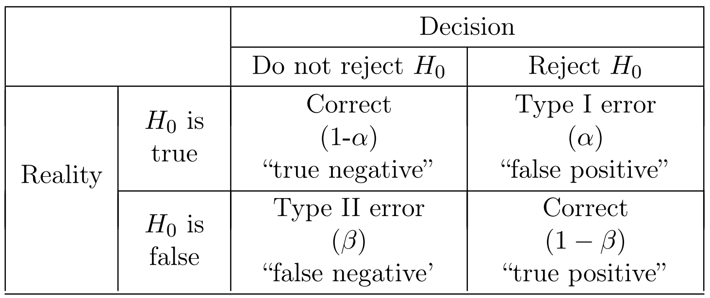
Since our decision is based on a random sample, there is always a chance of making a mistakenly false conclusion. There are two types of errors that can be made in carrying out a hypothesis testing.
Type I and type II erorrs with their probabilities \(\alpha\) and \(\beta\) respectively
Note that \(1-\beta\) is known as the power of the hypothesis test.
How to understand: fail to reject \(H_0\) and reject \(H_0\)
Note that in carrying out a hypothesis test, \(\alpha\) is typically specified, while power is not direcly controlled, but rather is influenced by the sample size and other factors.
An important point in terminology is that we don’t use the phrase “accept” for the null hypothesis, rather we “fail to reject it” (if we stick with \(H_0\)) or “reject it” (if we choose \(H_1\)). This is because when we fail to reject \(H_0\), we typically don’t know the actual value of \(\beta\), hence we aren’t able to put a level of certainty on \(H_0\) being the case. In other words, when we fail to reject \(H_0\), this doesn’t mean that \(H_0\) is true. We just haven’t enough evidence to reject it based on the sample data. This means that we are still likely to make type II error with the probability \(\beta\) (i.e. in reality, \(H_0\) is false, but we fail to reject it) though we fail to reject \(H_0\). Because we usualy don’t know the actual value of \(\beta\), we cannot give such an assertion that \(H_0\) is true with a specified confidence level. This is why we just say that we fail to reject \(H_0\) based on the sample data, instead of \(H_0\) is true.
However, if we do reject \(H_0\), then by the design of hypothesis tests we can say that our error probability is bounded by \(\alpha\).
8.9.1 How to design and perform a hypothesis testing
Formulate the scientific question as a hypothesis by partitioning the parameter space \(\Theta\) into \(\Theta_0\) and \(\Theta_1\), and then formimg the two hypotheses \(H_0 : \theta \in \Theta_0\) and \(H_1 : \theta \in \Theta_1\).
Define the test statistic, denoted \(X^*\), as a function of the sample data.
Since the test statistic follows some distribution under \(H_0\), the next step is to consider how likely it is to observe the specific value (\(X^*\)) calculated from the sample data under \(H_0\).
To this end, in setting up a hypothesis test, we typically choose a significance level \(\alpha\) (e.g. \(0.05\) or \(0.01\)), which quantifies our level of tolerance for enduring a type I error. For example, setting \(\alpha = 0.01\) implies we wish to design a test where the probability of type I error is at most\(0.01\) if \(H_0\) holds. Clearly, a low \(\alpha\) is desirable, however, there are tradeoffs involved since seeking a very low \(\alpha\) will imply a high \(\beta\) (low power).
Pick a significance level \(\alpha\).
Consider that we have a series of sample observations distributed as continuous uniform between \(0\) and some unknown upper bound \(m\).
Say we set
\[
H_0: m=1,\ \ \ \ H_1: m<1
\]
with observations \(X_1, ..., X_n\), one possible test statistic is the sample range:
As is always the case, the test statistic is a random variable. Under \(H_0\), we expect the distribution of \(X^*\) to have support \([0, 1]\) with the most likely value being close to \(1\). This is because low values of \(X^*\) are less plausible under \(H_0\). The explicit form of the distribution of \(X^*\) can be analytically obtained however for simplicity we use a Monte Carlo simulation to estimate it and present the density.
For this case, it is sensible to reject \(H_0\) if \(X^*\) is small enough.
Performing hypothesis testing.
At present, there are two alternatives for performing hypothesis tests:
Using rejection region:
Denoting quantiles of this distribution by \(q_0(u)\), then we set the rejection region as \(R = [0, q_0(\alpha)]\). Using Monte Carlo, we compute the rejection region where the critical value is the upper boundary \(q_0(\alpha)\) of the rejection region in this case. Note that computing the rejection region does not require any sample data as it is based on model assumptions and not the sample.
The decision rule for this hypothesis test is simple: compare the observed value of the test statistic, \(x^*\), to the critical value \(q_0(\alpha)\) and reject \(H_0\) if \(x^*\le q_0(\alpha)\), otherwise do not reject.
Using p-value:
We collect the data and compute the observed value of the test statistic \(x^*\). The p-value is then the maximal \(\alpha\) under which the test would be rejected with the observed test statistic. In other words, we find \(p\) which solves \(x^* = q_0(p)\). This is computed via \(F_0(x^*)\), where \(F(\cdot)\) is the CDF of \(X^*\).
Using the p-vaue approach, reporting a low p-value implies that we are very confident in rejecting \(H_0\), while a high p-value implies we are not. The p-value approach can be used to decide whether \(H_0\) should be rejected or not with a specified \(\alpha\). For this case, simply comparing \(p\) and \(\alpha\), and reject \(H_0\) if \(p\le \alpha\).
Using rejection region or p-value to perform hypothesis testing
usingDistributions, CairoMakie, Random, StatisticsRandom.seed!(1)n, N, alpha =10, 10^7, 0.05mActual =0.7dist0, dist1 =Uniform(0, 1), Uniform(0, mActual)ts(sample) =maximum(sample) -minimum(sample)empiricalDistUnderH0 = [ts(rand(dist0, n)) for _ in1:N]rejectionValue =quantile(empiricalDistUnderH0, alpha)samples =rand(dist1, n)testStat =ts(samples)pValue =sum(empiricalDistUnderH0 .<= testStat) / Nif testStat > rejectionValueprintln("Do not reject: ", round(testStat; digits=4), " > ", round(rejectionValue; digits=4))elseprintln("Reject: ", round(testStat; digits=4), " <= ", round(rejectionValue; digits=4))endprintln("p-value = ", round(pValue; digits=4))fig, ax =stephist(empiricalDistUnderH0; bins=100, color=:blue, normalization=:pdf)vlines!(ax, testStat; color=:red, label="Observed test statistic")vlines!(ax, rejectionValue; color=:black, label="Critical value boundary")axislegend(ax; position=:lt)ax.title = L"\text{The distribution of the test statistic }X^*\text{ under }H_0"fig
Reject: 0.5725 <= 0.6059
p-value = 0.032
8.9.2 Understand type I and type II errors
When the alternative parameter spaces \(\Theta_0\) and \(\Theta_1\) are only comprised of a single point each, the hypothesis test is called a simple hypothesis test.
Consider a container that conatins two identical types of pipes, except that one type weighs \(15\) grams on average and the other \(18\) grams on avearge. The standard deviation of the weights of both pipe types is \(2\) grams.
Imagine that we sample a single pipe, and wish to determine its type. Denote the weight of this pipe by the random variable \(X\). For this example, we devise the following statistical hypothesis test: \(\Theta_0 = {15}\) and \(\Theta_1 = {18}\). Now, given a threshold \(\tau\), we reject \(H_0\) if \(X > \tau\), otherwise we retain \(H_0\).
In this case, we can explicitly analyze the probabilities of both the type I and type II errors, \(\alpha\) and \(\beta\) respectively.
usingDistributions, StatsBase, CairoMakiemu0, mu1, sd, tau =15, 18, 2, 17.5dist0, dist1 =Normal(mu0, sd), Normal(mu1, sd)grid =5:0.1:25h0grid, h1grid = tau:0.1:25, 5:0.1:tau# CCDF: complementary CDFprintln("Probability of Type I error: ", ccdf(dist0, tau))println("Probability of Type II error: ", cdf(dist1, tau))fig, ax =lines(grid, pdf.(dist0, grid); color=:red, label="Bolt type 15g")band!(ax, h0grid, repeat([0], length(h0grid)), pdf.(dist0, h0grid); color=(:red, 0.2))lines!(ax, grid, pdf.(dist1, grid); color=:green, label="Bolt type 18g")band!(ax, h1grid, repeat([0], length(h1grid)), pdf.(dist1, h1grid); color=(:green, 0.2))linesegments!(ax, [tau, 25], [0, 0]; color=:black, label="Rejection region", linewidth=5)text!([15, 18, 15.5, 18.5], [0.21, 0.21, 0.02, 0.02]; text=[L"H_0", L"H_1", L"\beta", L"\alpha"], align=repeat([(:center, :center)], 4), fontsize=28)axislegend(ax)fig
Probability of Type I error: 0.10564977366685525
Probability of Type II error: 0.4012936743170763
8.9.3 The Receiver Operating Curve (ROC)
In the previous example, \(\tau = 17.5\) was arbitrarily chosen.
Clearly, if \(\tau\) was increased, the probability of making a type I error, \(\alpha\), would decrease, while the probability of making a type II error, \(\beta\), would increase. Conversely, if we decreased \(\tau\) the reverse would occur.
Here we use the Receiver Operating Curve (ROC) to help to visualize the tradeoff between type I and type II errors. It allows us to visualize the error tradeoffs for all possible \(\tau\) values simutaneously for a particular alternative hypothesis \(H_1\).
Below we plot the analytic coordinates of \((\alpha(\tau), 1-\beta(\tau))\). This is the ROC. It is a parametric plot of the probability of a type I error and power.
We now investigate the concept of a randomization test, which is a type of non-parametric test, i.e. a statistical test which does not require that we know what type of distribution the data comes from.
A virtue of non-parametric tests is that they do not impose a specific model.
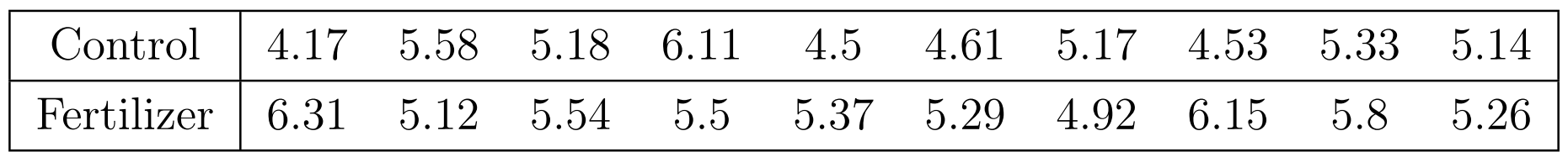
Consider the following example, where a farmer wants to test whether a new fertilizer is effective at increasing the yield of her tomato plants. As an experiment, she took \(20\) plants, kept \(10\) as controls, and treated the remaining \(10\) with fertilizer, After \(2\) months, she harvested the plants and recorded the yield of each plant in kg as shown in the following table:
Yield in kg for \(10\) plants with, and \(10\) plants without fertilizer (control)
It can be observed that the group of plants treated with fertilizer have an average yield \(0.494\) kg greater than that of the control group. One could argue that this difference is due to the effects of the fertilizer. We now investigate if this is a reasonable assumption. Let us assume for a moment that the fertilizer had no effect on plant yield (\(H_0\)) and that the result was simply due to random chance. In such a scenario, we actually have \(20\) observations from the same group, and regardless of how we arrange our observations, we would expect to observe similar results.
Hence, we can investigate the likelihood of this outcome occurring by random chance, by considering all possible combinations of \(10\) samples from our group of \(20\) observations, and counting how many of these combinations result in a difference in sample means greater than or equal to \(0.494\) kg. The proportion of times this occurs is analogous to the likelihood that the difference we observe in our sample means was purely due to random chance. It is in a sense the p-value.
Before proceeding, we calculate the number of ways one can sample \(r = 10\) unique items from \(n = 20\) total, which is given by
\[
\binom{20}{10} = 184,756
\]
Hence, the number of possible combinations in our example is computationally manageable. Note that in a different situation where \(n\) and \(r\) would be bigger, e.g. \(n = 40\) and \(r = 20\), the number of combinations would be too big for an exhaustive search (about \(137\) billion). In such a case, a viable alternative is to randomly sample combinations for estimating the p-value.
usingCombinatorics, Statistics, DataFrames, CSVdf = CSV.read("./data/fertilizer.csv", DataFrame)control = df.Controlfertilizer = df.FertilizerXsubGroups =collect(combinations([control; fertilizer], 10))meanFert =mean(fertilizer)pVal =sum([mean(i) >= meanFert for i in subGroups]) /length(subGroups)println("p-value = ", pVal)
p-value = 0.023972157873086666
8.10 Bayesian statistics
In the Bayesian paradigm, the scalar or vector of parameter \(\theta\) is not assumed to exist as some fixed unknown quantity but instead is assumed to follow a distribution.
That is, the parameter itself, is a random variable, and the act of Bayesian inference is the process of obtaining more information about the distribution of \(\theta\).
This allows us to incorparate prior beliefs about the parameter before experience from new observations is taken into consideration.
The key objects at play are the prior distribution of the parameter and the posterior distribution of the parameter.
The former is postulated beforehand, or exists as a consequence of previous inference, while the latter captures the distribution of the parameter after observations are taken into consideration.
The relationship between the prior and the posterior is
This is nothing but Bayes’s rule \(P(B_i|A) = \frac{P(A|B_i)P(B_i)}{\sum_{j=1}^{n}P(A|B_j)P(B_j)}, A\in \cup_{i=1}^n B_i\) applied to densities.
Here the prior distribution (density) is \(f(\theta)\), and the posterior distribution (density) is \(f(\theta|x)\).
Observe that the denominator, known as evidence or marginal likelihood, is constant with respect to the parameter \(\theta\). This allows the equation to be written as
Hence, the posterior distribution can be easily obtained up to the normalizing constant (the evidence) by multiplying the prior with the likelihood.
In general, carrying out Beyesian inference involves the following steps:
Assume some distributional model for the data based on the parameter \(\theta\) which is a random variable.
Use previous inference experience, elicit an expert, or make an educated guess to determine a prior distribution \(f(\theta)\). The prior distribution might be parameterized by its own parameters, called hyper-parameters.
Collect data \(x\) and create an expression or a computational mechanism for the likelihood \(f(x|\theta)\) based on the distributional model chosen.
Use the Bayes’s rule applied to densities to obtain the posterior distribution of the parameters \(f(\theta|x)\).
In most cases, the evidence (the denominator) is not easily computable. Hence the posterior distribution is only available up to a normalizing constant. In some special cases, the form of the posterior distribution is the same as the prior distribution. In such cases, conjugacy holds, the prior is called a conjugate prior, and the hyper-parameters are updated from prior to posterior.
The posterior distribution can then be used to make conclusions about the model.
For example, if a single specific parameter value is needed to make the model concrete, a Bayes estimate based on the posterior distribution, for example, the posterior mean, may be computed:
Further analyses such as obtaining credible intervals, similar to condidence intervals, may also be carried out.
The model with \(\hat{\theta}\) can then be used for making conclusions. Alternatively, a whole class of models based on the posterior distribution \(f(\hat{\theta}|x)\) can be used. This often goes hand in hand with simulation as one is able to generate Monte Carlo samples from the posterior distribtion.
8.10.1 A Poisson example
Consider an example where an insurance company models the number of weekly fires in a city using a Poisson distribution with parameter \(\lambda\). Here, \(\lambda\) is also the expected number of fires per week.
Assume that the following data is collected over a period of \(16\) weeks:
Each data point indicates the number of fires per week.
In this case, the MLE is \(\hat{\lambda} = 1.8125\) simply obtained by the sample mean. Hence, in a frequentist approach, after \(16\) weeks, the distribution of the number of fires per week is modeled by a Poisson distribution with \(\lambda = 1.8125\). One can then obtain estimates for say, the probability of having more than \(5\) fires in a given week as follows:
However, the drawback of such an approach in estimating \(\lambda\) is that it didn’t make use of previous information.
Say that for example, further knowledge comes to light that the number of fires per week ranges between \(0\) and \(10\), and that the typical number is \(3\) fires per week. In this case, one can assign a prior distribution to \(\lambda\) that captures this belief.
In this example, we can assume that we decide to use a triangular distribution which captures prior beliefs about the parameter \(\lambda\) well because it has a defined range and a defined mode.
With the prior assigned and the data collected, we can use the machinery of Bayesian inference.
In this case, the prior distibution of the parameter \(\lambda\) is the triangular distribution with the PDF:
The gamma distribution is said to be a conjugate prior to the Poisson distribution, which means that both the prior distribution and the posterior distribution are gamma distributions when the data is distributional as a Poisson distribution. In this case, the hyper-parameters typically have a simple update law from prior to posterior.
In the case of a gamma-Poisson conjugate pair, assume the hyper-parameters of the prior to have \(\alpha\) (shape parameter) and \(\beta\) (rate parameter). We have
Computational Bayes Estimate: 2.055555555555556
Closed form Bayes Estimate: 2.0555555555555554
8.10.3 Markov Chain Monte Carlo example
In cases where the dimension of the parameter space is high, carrying out straighforward integration is not possible.
However, there are other ways of carrying out Bayesian inference.
One such popular way is by using algorithms that fall under the category known as Markov Chain Monte Carlo (MCMC).
The Metropolis-Hastings algorithm is one such popular MCMC algorithm.
It produces a series of samples \(\theta(1), \theta(2), \theta(3), ...\), where it is guaranteed that for large \(t\), \(\theta(t)\) is distributed according to the posterior distribution.
Technically, the random sequence \(\{\theta(t)\}_{t=1}^\infty\) is a Markov chain and it is guaranteed that the stationary distribution of this Markov chain is the specified posterior distribution. That is, the posterior distribution is an input parameter to the algorithm.
The major bebefits of Metropolis-Hastings and similar MCMC algorithms is that they only use the ratios of the posterior on different parameter values. For example, for parameter \(\theta_1\) and \(\theta_2\), the algorithm only uses the posterior distribution via the ratio
This means that the normalizing constant (evidence) is not needed as it is implicitly canceled out. Thus, using \(\text{psoterior} \propto \text{likelihood}\times \text{prior}\) suffices.
Further to the posterior distribution, an additional input parameter to Metropolis-Hastings is the so-called proposal density, denoted by \(q(\cdot|\cdot)\). This is a family of distributions where given a certain value of \(\theta_1\) taken as a parameter, the new value, say \(\theta_2\) is distributed with PDF
\[
q(\theta_2|\theta_1)
\]
The idea of Metropolis-Hastings is to walk around the parameter space by randomly generating new values using \(q(\cdot|\cdot)\).
At each step, some new values are accepted while others are not, all in a manner which ensures the desired limiting behavior. The algorithm specification is to accept with probability
\[
H = \min\left\{1,\ L(\theta^*, \theta(t)) \frac{q(\theta(t)|\theta^*)}{q(\theta^*|\theta(t))}\right\}
\]
where \(\theta^*\) is the new proposed value, generated via \(q(\cdot|\theta(t))\), and \(\theta(t)\) is the current value.
With each such iteration, the new value is accepted with probability \(H\) and rejected otherwise. With certian technical requirements on the posterior and proposal densities, the theory of Markov chains then guarantees that the stationary distribution of the sequence \(\{\theta(t)\}\) is the posterior distribution.
Different variants of the Metropolis-Hastings algorithm employ different types of proposal densities. There are also generalizations and extensions that we don’t discuss here, such as Gibbs Sampling and Hamiltonian Monte Carlo.
As an example, we use the folded normal distribution as a proposal density. This distribution is achieved by taking a normal random variable \(X\) with mean \(\mu\) and variance \(\sigma^2\) and considering \(Y=|X|\). In this case, the PDF of \(Y\) is
It supports to generate the non-negative parameters in question.
usingDistributions, CairoMakiealpha, beta =8, 2# prior with Gamma distribution which has two hyper-parameters α and βprior(lam) =pdf(Gamma(alpha, 1/ beta), lam)d = [2, 1, 0, 0, 1, 0, 2, 2, 5, 2, 4, 0, 3, 2, 5, 0]# data with Poisson distribution which has a parameter λlike(lam) =*([pdf(Poisson(lam), x) for x in d]...)# posterior ∝ likelihood * priorposteriorUpToK(lam) =like(lam) *prior(lam)sig =0.5# use the folded normal distribution as the proposal density# with each parameter θ1, it produces a new parameter θ2foldedNormalPDF(x, mu) = (1/sqrt(2*pi* sig^2)) * (exp(-(x - mu)^2/2sig^2) +exp(-(x + mu)^2/2sig^2))foldedNormalRV(mu) =abs(rand(Normal(mu, sig)))functionsampler(piProb, qProp, rvProp) lam =1 warmN, N =10^5, 10^6 samples =zeros(N - warmN)for t in1:Nwhiletrue lamTry =rvProp(lam) Lo =piProb(lamTry) /piProb(lam) H =min(1, Lo *qProp(lam, lamTry) /qProp(lamTry, lam))ifrand() < H lam = lamTryif t > warmN samples[t-warmN] = lamendbreakendendendreturn samplesendmcmcSamples =sampler(posteriorUpToK, foldedNormalPDF, foldedNormalRV)println("MCMC Bayes Estimate: ", mean(mcmcSamples))fig, ax =stephist(mcmcSamples; bins=100, color=:black, normalization=:pdf, label="Histogram of MCMC samples")lamRange =0:0.01:10lines!(ax, prior.(lamRange); color=:blue, label="Prior distribution")closedFormPosterior(lam) =pdf(Gamma(alpha +sum(d), 1/ (beta +length(d))), lam)lines!(ax, lamRange, closedFormPosterior.(lamRange); color=:red, label="Posterior distribution")ax.limits = (0, 10, 0, 1.2)ax.xlabel = L"\lambda"ax.ylabel ="Density"axislegend(ax)fig
MCMC Bayes Estimate: 2.066064798662241
9 Confidence intervals
In the setting of symmetric sampling distributions, a typical formula for the confidence interval \([L, U]\) is of the form
\[
\hat{\theta} \pm K_\alpha s_\text{err}
\]
Here, \(\hat{\theta}\) is typically the point estimate for the parameter in question, \(s_\text{err}\) is some measure or estimate of the variability (e.g. standard error) of the parameter, and \(K_\alpha\) is a constant which depends on the model at hand and on \(\alpha\). Typically by decreasing \(\alpha \rightarrow 0\), we have that \(K_\alpha\) increases, implying a wider confidence interval. In addition, the specific form of \(K_\alpha\) often depends on conditions such as
Sample size: is the sample size small or large.
Variance: is the variance \(\sigma^2\) known or unknown.
Distribution: is the population assumed normally distributed or not.
9.1 Single sample confidence intervals for the mean
Assume that we want to estimate the population mean \(\mu\) using a random sample, \(X_1, ..., X_n\).
As mentioned before, an unbiased point estimate for the mean is the sample mean \(\overline{X}\), so a typical formula for the confidence interval of the mean is
If we assume that the population variance \(\sigma^2\) is known and the data is normally distributed, then the sample mean \(\overline{X}\) is normally distributed with mean \(\mu\) and variance \(\frac{\sigma^2}{n}\). This yields
In practice, \(\sigma^2\) is rarely known; hence, it is tempting to replace \(\sigma\) by \(s\) (sample standard deviation) in the formula above. Such a replacement is generally fine for large samples.
In addition, the validity of the normality assumption should also be considered. In cases where the data is not normally distributed, the probability statement above only approximately holds. However, as \(n \rightarrow \infty\), it quickly becomes precise due to the central limit theorem.
usingDistributions, HypothesisTestsd = [53.35674558144255,53.45887516134873,52.282838627926125,52.98746570643515,51.993167774733486,53.373333606198,55.75410538860477,50.279496381439365,53.6359586914001,53.517705831707495,53.70044994508253,54.15592592604583,53.55054914606446,52.37319589109419,53.4900750059897,52.939458524079605,52.16761562743534,50.87140009591033,53.144919157924924,52.09084035473537,]xBar, n =mean(d), length(d)sig =1.2alpha =0.1z =quantile(Normal(), 1- alpha /2)println("Calculating formula: ", (xBar - z * sig /sqrt(n), xBar + z * sig /sqrt(n)))println("Using confint() function: ", confint(OneSampleZTest(xBar, sig, n); level=1- alpha))
Calculating formula: (52.514845578531826, 53.39756666402797)
Using confint() function: (52.514845578531826, 53.39756666402797)
Note
Assume \(U \sim N(0, 1)\), and \(X \sim N(\mu, \sigma)\), we have
\[
U = \frac{X-\mu}{\sigma}
\]
\[
X = \mu + U\sigma
\]
\[
P(-z_{1-\frac{\alpha}{2}} \le U \le z_{1-\frac{\alpha}{2}}) = 1-\alpha
\]
In cases where the population variance is unknown, if we replace \(\sigma\) by the sample standard deviation \(s\), we can use the T-distribution instead of the normal distribution to obtain the confidence interval for the mean
where \(t_{1-\frac{\alpha}{2}, n-1}\) is the \(1-\frac{\alpha}{2}\) quantile of a T-distribution with \(n-1\) degrees of freedom.
For small samples, the replacement of \(z_{1-\frac{\alpha}{2}}\) by \(t_{1-\frac{\alpha}{2}, n-1}\) significantly affects the width of the confidence interval, as for the same value of \(\alpha\), the T case is wider.
However, as \(n \rightarrow \infty\), we have, \(t_{1-\frac{\alpha}{2}, n-1} \rightarrow z_{1-\frac{\alpha}{2}}\).
usingDistributions, HypothesisTestsd = [53.35674558144255,53.45887516134873,52.282838627926125,52.98746570643515,51.993167774733486,53.373333606198,55.75410538860477,50.279496381439365,53.6359586914001,53.517705831707495,53.70044994508253,54.15592592604583,53.55054914606446,52.37319589109419,53.4900750059897,52.939458524079605,52.16761562743534,50.87140009591033,53.144919157924924,52.09084035473537,]xBar, n =mean(d), length(d)s =std(d)alpha =0.1t =quantile(TDist(n -1), 1- alpha /2)println("Calculating formula: ", (xBar - t * s /sqrt(n), xBar + t * s /sqrt(n)))println("Using confint() function: ", confint(OneSampleTTest(xBar, s, n); level=1- alpha))
Calculating formula: (52.499893857795534, 53.41251838476426)
Using confint() function: (52.499893857795534, 53.41251838476426)
9.2 Two sample confidence intervals for the difference in means
It is often of interest to estimate the difference between the population means, \(\mu_1 - \mu_2\).
First we collect two random samples, \(x_{i,1}, ..., x_{i,n}\) for \(i = 1,2\), each with the sample mean \(\bar{x}_i\) and sample standard deviation \(s_i\). In addition, the difference of sample means, \(\bar{x}_1 - \bar{x}_2\) serves as a point estimate for the difference in population means, \(\mu_1 - \mu_2\).
A confidence interval for \(\mu_1 - \mu_2\) around the point estimate \(\bar{x}_1 - \bar{x}_2\) is then constructed via the same process seen previously
9.2.2 Population variances unknown and assumed equal
In cases where the population variances are unknown but assumed equal, denoted by \(\sigma^2\). Based on this assumption, it is sensible to use both sample variances to estimate \(\sigma^2\). This estimated variance using both samples is known as the pooled sample variance, and is given by
Calculating formula: (1.0960161140340268, 2.9216026985257764)
Using confint() function: (1.0960161140340265, 2.921602698525777)
9.2.4 More on the Satterthwaite approximation
Observe that both sides of the “distributed as” (\(\sim\)) symbol are random variables which depdend on the same random experiment.
Hence, the statement can be presented generally, as a case of the following format:
\[
X(\omega) \sim F_{h(\omega)}
\]
where \(\omega\) is a point in the sample space.
Here, \(X(\omega)\) is a random variabe, and \(F\) is a distribution that depends on a parameter \(h\), which depends on \(\omega\).
In our case of the Satterthwaite approximation, \(h\) is \(v\), defined above.
Why both sides of the \(\sim\) symbol are random variables which depend on the same random experiment
When we had finished a random experiment, we obtained a sample \(\omega\) from the sample space.
Then, we can derive some statistic (\(X(\omega)\)) from the sample, which means that \(X\) is a random variable. In addition, under the same experiment, \(X\) should be distributed as some distribution \(F\), which may be defined by some parameter \(h\), saying the degrees of freedom. Obviously, \(h\) itself depends on the same sample obtained from the sample space before.
By using the inverse probability transformation, the above formula is equivalent to
This means that the Satterthwaite approximation is a better approximative distribution close to the true distribution which \(T\) calculated in the case of population variances unknown and not assumed equal is distributed as in comparison with the alternative of treating \(h\) as simply dependent on the number of observations made (\(n_1+n_2-2\)).
We can make a simple validation using Q-Q plot: \(t(v)\) is more similar with the true distribution of \(T\) than \(t(n_1+n_2-2)\)
In certain inference settings the parameter of interest is a population proportion.
When carrying out inference for a proportion we assume that there exists some unknown population proportion \(p \in (0, 1)\).
We then sample an i.i.d. sample of observations \(I_1, ..., I_n\), where for the \(i\)’th observation, \(I_i = 0\) if the event in question does not happen, and \(I_i = 1\) if the event occurs.
A natural estimator for the proportion is then the sample mean of \(I_1, ..., I_n\), which we denote
\[
\hat{p} = \frac{\sum_{i=1}^{n}I_i}{n}
\]
Please note that \(\overline{X} \sim N(\mu, \frac{\sigma^2}{n})\) as \(n \rightarrow \infty\), so is \(\hat{p}\).
Now observe that each \(I_i\) is a Bernoulli random variable with success probability \(p\). Under the i.i.d assumption this means that the numerator of the above formula (i.e. \(\sum_{i=1}^{n}I_i\)) is binomially distributed with parameters \(n\) and \(p\). Hence
\[
E\left[\sum_{i=1}^{n}I_i\right] = np
\]
and
\[
\text{Var}(\sum_{i=1}^{n}I_i) = np(1-p)
\]
So we have
\[
E(\hat{p}) = p
\]
and
\[
\text{Var}(\hat{p}) = \frac{p(1-p)}{n}
\]
Hence, \(\hat{p}\) is an unbiased and consistent estimator of \(p\). That is, on average\(\hat{p}\) estimates \(p\) perfectly (unbiased), and if more observations are collected the variance of the estimator vanishes and then \(\hat{p} \rightarrow p\) (consistent).
Furthermore, we can use the central limit theorem to create a normal approximation for the distribution of \(\hat{p}\) and yield an approximate condidence interval.
Due to the fact \(\hat{p} \sim N(p, \frac{p(1-p)}{n})\) as \(n \rightarrow \infty\), we have
which is a random variable that approximately follows a standard normal distribution. The approximation becomes exact as \(n\) grows. Due to the fact that \(\hat{p}\) is an unbiased and consistent estimator of \(p\), it’s reasonable that we replace \(p\) with \(\hat{p}\), and then we have
usingCSV, DataFrames, CategoricalArrays, Distributionsdat = CSV.read("./data/purchaseData.csv", DataFrame)println("Levels of Grade: ", levels(dat.Grade))println("Data points: ", nrow(dat))n =sum(.!(ismissing.(dat.Grade)))println("Non-missing data points: ", n)dat2 =dropmissing(dat[:, [:Grade]], :Grade)gradeInQuestion ="E"indicatorVector = dat2.Grade .== gradeInQuestionnumSuccess =sum(indicatorVector)phat = numSuccess / nserr =sqrt(phat * (1- phat) / n)alpha =0.05confidencePercent =100* (1- alpha)zVal =quantile(Normal(), 1- alpha /2)confInt = (phat - zVal * serr, phat + zVal * serr)println("\nOut of $n non-missing observations, $numSuccess are at level $gradeInQuestion.")println("Hence a point estimate for the proportion of grades at level $gradeInQuestion is $phat.")println("A $confidencePercent% confidence interval for the proportion of level $gradeInQuestion is:\n$confInt")
Levels of Grade: String1["A", "B", "C", "D", "E"]
Data points: 200
Non-missing data points: 187
Out of 187 non-missing observations, 61 are at level E.
Hence a point estimate for the proportion of grades at level E is 0.32620320855614976.
A 95.0% confidence interval for the proportion of level E is:
(0.2590083767381328, 0.3933980403741667)
9.3.1 Sample size planing
Denote the confidence interval of the proportion as \(\hat{p} \pm E\) where \(E\) is the margin of error or half the width of the confidence interval, denoted by
\[
E = z_{1-\frac{\alpha}{2}}\sqrt{\frac{\hat{p}(1-\hat{p})}{n}}
\]
We may often want to plan an experiment or a sampling scheme such that \(E\) is not too wide.
Say we want \(E \le \epsilon\) with the confidence probability \(1-\alpha\), we have
\[
E = z_{1-\frac{\alpha}{2}}\sqrt{\frac{\hat{p}(1-\hat{p})}{n}} \le \epsilon
\]
Given that \(x(1-x)\) is maximized at \(x=1/2\) with a maximal value of \(1/4\). Hence,
\[
E \le \frac{z_{1-\frac{\alpha}{2}}}{2\sqrt{n}} \le \epsilon
\]
Finally, we have
\[
n \ge \frac{z_{1-\frac{\alpha}{2}}^2}{4\epsilon^2}
\]
9.3.2 Validity of the approximation
In many cases, this confidence interval approximation for the proportion works well, however for small sample sizes \(n\) or values of \(p\) near \(0\) or \(1\), this is often too crude of an approximation. A consequence is that one may obtain a confidence interval that isn’t actually a \(1-\alpha\) confidence interval, but rather has a different coverage probability.
One common rule of thumb used to decide if the confidence interval for the proportion is valid is to require that both the product \(np\) and the product \(n(1-p)\) be at least \(10\).
Here, we expore some combinations of \(n\) and \(p\). For each combination, we use \(N\) Monte Carlo expriments and calculate the following
This estimated difference of the actual converage probability of the confidence interval and the desired confidence level \(1-\alpha\) is a measure of the accuracy of the confidence level. We expect this difference to be almost \(0\) if the approximation is good. Otherwise, a higher absolute difference is oberved.
usingRandom, Distributions, CairoMakieN =5e3alpha =0.05confLevel =1- alphaz =quantile(Normal(), 1- alpha /2)functionrandCI(n, p) sample =rand(n) .< p pHat =sum(sample) / n serr =sqrt(pHat * (1- pHat) / n) (pHat - z * serr, pHat + z * serr)endcover(p, ci) = ci[1] <= p && p <= ci[2]pGrid =0.1:0.01:0.9nGrid =5:1:50errs =zeros(length(nGrid), length(pGrid))for i in1:length(nGrid)for j in1:length(pGrid)Random.seed!(1234) n, p = nGrid[i], pGrid[j] coverageRatio =sum([cover(p, randCI(n, p)) for _ in1:N]) / N errs[i, j] = confLevel - coverageRatioendendfig, ax1, hm1 =heatmap(pGrid, nGrid, errs'; colormap=to_colormap(["white", "black"]))ax2, hm2 =heatmap(fig[2, 1], pGrid, nGrid, errs'.<=0.04; colormap=to_colormap(["black", "white"]))Colorbar(fig[1, 2], hm1)fig
9.4 Confidence interval for the variance of a normal population
First, a point estimator of the population variance is the sample variance
We have known that \(\frac{(n-1)s^2}{\sigma^2} \sim \chi_{n-1}^2\). So denoting the \(\gamma\)-quantile of this distribution via \(\chi_{\gamma,n-1}^2\), we have
Note: this equality holds only if the data is normally distributed.
usingDistributionsdat =rand(Normal(0, 1), 1000)n, s, alpha =length(dat), std(dat), 0.05ci = ((n -1) * s^2/quantile(Chisq(n -1), 1- alpha /2), (n -1) * s^2/quantile(Chisq(n -1), alpha /2))println("Point estimate for the variance: ", s^2)println("Confidence interval for the variance: ", ci)
Point estimate for the variance: 0.9999905881991535
Confidence interval for the variance: (0.9177790230416273, 1.0938240508530526)
9.4.1 Sensitivity of the normal assumption
As mentioned before, this confidence interval for the variance of a normal population only holds for normally distributed population and is more sensitive about the normal assumption than the other confidence intervals constructed before.
We’ll find that the sample variance distributions of a normal distribution and a logistic distribution are quite different, though they have the same pupulation mean \(\mu\) and population variance \(\sigma^2\), and the PDF’s curve shape of the logistic distribution is somewhat similar with the normal.
The logistic distribution is defined by the location and scale parameters \(\mu\) and \(\eta\), and the PDF is
In addition, we can check the actual confidence interval coverage under different model assumptions:
usingDistributions, CairoMakiemu, sig =2, 3eta =sqrt(3) * sig /pin, N =15, 10^4dNormal =Normal(mu, sig)dLogistic =Logistic(mu, eta)alphaUsed =0.001:0.001:0.1functionalphaSimulator(dist, n, alpha) popVar =var(dist) coverageCount =0for _ in1:N sVar =var(rand(dist, n)) Lo = (n -1) * sVar /quantile(Chisq(n -1), 1- alpha /2) Up = (n -1) * sVar /quantile(Chisq(n -1), alpha /2) coverageCount += Lo < popVar && popVar < Upend1- coverageCount / Nendfig, ax =ablines(0, 1; color=:green, label="y = x")scatter!(ax, alphaUsed, alphaSimulator.(dNormal, n, alphaUsed); color=:blue, label="Normal")scatter!(ax, alphaUsed, alphaSimulator.(dLogistic, n, alphaUsed); color=:red, label="Logistic")axislegend(ax; position=:lt)fig
9.5 Bootstrap confidence intervals
Bootstrap, also called empirical bootstrap, is a useful technique which relies on resampling from the observed data \(x_1, ..., x_n\)with replacement in order to empirically construct the distribution of the point estimator for some unknown population parameters.
One way in which this resampling can be conducted is to apply the inverse probability transform on the empirical cumulative distribution function.
Note
Obtain a sample: \(\mathbf{X} = (x_1, ..., x_n)\).
Obtain the empirical cumulative distribution function \(F_X(\mathbf{X})\) based on \(\mathbf{X}\).
Use the inverse probability transformation: \(\mathbf{U} = F_X(\mathbf{X}) \Longrightarrow \mathbf{X} = F_X^{-1}(\mathbf{U})\).
Resample \(\mathbf{X}\) via resampling \(\mathbf{U} \sim U(0, 1)\) with replacement.
It seems that we sample a large number of “new” samples from the population, and then we can get a large number of point estimators, which then are used to construct the empirical distribution of the point estimator. Finally, to get the \(1-\alpha\) confidence interval, we can just get the quantiles of \(\frac{\alpha}{2}\) and \(1-\frac{\alpha}{2}\).
Bootstrap requires that the number of observations is not too small.
However, from an implementation perspective, a simpler alternative is to consider the data points \(x_1, ..., x_n\), and then randomly sample \(n\) discrete uniform indexes, \(j_1, ..., j_n\) each in the range \(\{1, ..., n\}\). The resampled data denoted by \(x^* = (x_1^*, ..., x_n^*)\) is then
\[
x^* = (x_{j_1}, ..., x_{j_n})
\]
That is, each point in the resampeld data is a random observation from the original data, where we allow to sample with replacement.
In Julia, \(x^* = \text{rand}(\mathbf{X}, n)\), where we use the rand() method to uniformally sample \(n\) random copies of elements in \(\mathbf{X}\) with replacement.
The idea of empirical bootstrap is now to repeat the resampling a large number of times, say \(N\), and for each resampled data vector, \(x^*(1), ..., x^*(N)\) to compute the parameter estimate. If the parameter estimate is denoted by the function \(h: R^n \mapsto R\), then we end up with values
Finally, a bootstrap confidence interval is determined by computing the respective lower and upper \((\frac{\alpha}{2}, 1-\frac{\alpha}{2})\) quantiles of the sequence \(h^*(1), ..., h^*(N)\).
usingRandom, Distributions, CairoMakieRandom.seed!(0)sampleData = [53.35674558144255,53.45887516134873,52.282838627926125,52.98746570643515,51.993167774733486,53.373333606198,55.75410538860477,50.279496381439365,53.6359586914001,53.517705831707495,53.70044994508253,54.15592592604583,53.55054914606446,52.37319589109419,53.4900750059897,52.939458524079605,52.16761562743534,50.87140009591033,53.144919157924924,52.09084035473537,]n, N =length(sampleData), 10^6alpha =0.1# sampling with replacementbootstrapSampleMeans = [mean(rand(sampleData, n)) for _ in1:N]Lmean =quantile(bootstrapSampleMeans, alpha /2)Umean =quantile(bootstrapSampleMeans, 1- alpha /2)println("Bootstrap confidence interval for the mean: ", (Lmean, Umean))fig, ax =stephist(bootstrapSampleMeans; bins=1000, color=:blue, normalization=:pdf, label="Sample means")vlines!(ax, [Lmean, Umean]; color=:red, label="90% CI")axislegend(ax)fig
Bootstrap confidence interval for the mean: (52.52963545344743, 53.375601378187525)
Simply, we can carry out a computational experiment to show that if the number of sample observations is not very large, then the coverage probability of bootstrapped confidence interval is only approximately \(1-\alpha\), but not exactly. However, as the sample size \(n\) grows, the coverage probability converges to the desired \(1-\alpha\).
usingRandom, DistributionsRandom.seed!(0)lambda =0.1dist =Exponential(1/ lambda)actualMedian =median(dist)M =10^3N =10^4nRange =2:2:20alpha =0.05for n in nRange coverageCount =0for _ in1:M sampleData =rand(dist, n) bootstrapSampleMeans = [median(rand(sampleData, n)) for _ in1:N] Lo =quantile(bootstrapSampleMeans, alpha /2) Up =quantile(bootstrapSampleMeans, 1- alpha /2) coverageCount += Lo < actualMedian && actualMedian < Upendprintln("n = ", n, "\t coverage = ", coverageCount / M)end
n = 2 coverage = 0.499
n = 4 coverage = 0.889
n = 6 coverage = 0.942
n = 8 coverage = 0.924
n = 10 coverage = 0.936
n = 12 coverage = 0.934
n = 14 coverage = 0.943
n = 16 coverage = 0.945
n = 18 coverage = 0.954
n = 20 coverage = 0.927
9.6 Prediction intervals
A prediction interval tells us a predicted range that a single next observation of data is expected to fall within with some level of confidence. This differs from a confidence interval which indicates how confident we are of a particular parameter that we are trying to estimate.
In brief, a prediction interval is constructed based on the distribution of a population itself from which we sample observations, while a confidence interval is constructed based on the distribution of a particular parameter which we are trying to estimate (e.g. \(\overline{X} \sim N(\mu, \frac{\sigma^2}{n})\)).
Suppose we have a sequence of data points (observations) \(x_1, x_2, x_3, ...\), which come from a normal distribution and are assumed i.i.d. Further assume that we observed the first \(n\) data points \(x_1, ..., x_n\), but have not yet observed \(X_{n+1}\). Note that we use lower case \(x\) for values observed and upper case \(X\) for yet unobserved random variables.
In this case, a \(1-\alpha\) prediction interval for the single future observation \(X_{n+1}\) is given by
and finally has an expected width close to \(2z_{1-\frac{\alpha}{2}}\sigma\).
Note
Suppose \(X\) is a normally distributed variable (i.e. \(X \sim N(\mu, \sigma^2)\)), and then we have \(U = \frac{X-\mu}{\sigma} \sim N(0, 1)\).
For \(U\), we have a \(1-\alpha\) prediction interval \(-z_{1-\frac{\alpha}{2}} \le U \le z_{1-\frac{\alpha}{2}}\), and then we have \(\mu - z_{1-\frac{\alpha}{2}}\sigma \le X \le \mu + z_{1-\frac{\alpha}{2}}\sigma\), which is a \(1-\alpha\) prediction interval of \(X\) in the case of population mean and population variance known.
Simply, a prediction interval is such an interval constructed based on the distribution of observations and needs to cover a \(1-\alpha\) proportion of this distribution.
The concept of credible intervals comes from the field of Bayesian statistics.
In general, we often need to find an interval \([l, u]\) such that given some probability density \(f(x)\), the interval satisfies
\[
\int_l^u f(x)dx = 1-\alpha
\]
This is needed for confidence intervals, prediction intervals, and credible intervals.
However, as long as \(\alpha < 1\), there is more than one interval \([l, u]\) that satisfies the above formula.
In certain cases, there is a “natural” interval. For example, for a symmetric distribution, using equal quantiles is natural (i.e. \(l = z_{\frac{\alpha}{2}}\) and \(u = z_{1-\frac{\alpha}{2}}\)). In such cases, the mean is also the median and further if the density is unimodal (has a single maximum) the mean and median are also the mode.
However, consider asymmetric distribution, there isn’t an immediate “natrual” choice for \(l\) and \(u\). There are three types of intervals we often use:
Classic interval: this type of interval has the mode of the density (assuming the density is unimodal) at its center between \(l\) and \(u\). An alternative is to use mean or median at the center. That is, assuming the centrality measure (mode, mean, or median) is \(m\), we have \([l, u] = [m-E, m+E]\). One way to define \(E\) is via
Equal tail interval: this type of interval simply sets \(l\) and \(u\) as the \(\frac{\alpha}{2}\) and \(1-\frac{\alpha}{2}\) quantiles, respectively. Namely,
Highest density interval: this type of interval seeks to cover the part of the support that is most probable. A consequence is that if the density is unimodal then this highest density interval is also the narrowest possible confidence interval. We can crudely does so by starting with a high-density value and decreasing it gradually while seeking for the associated interval \([l, u]\). An alternative would be to gradually increment \(l\) each time finding a corresponding \(u\) that satisfies the above formula and within this search to choose the interval that minimizes the width \(u-l\).
For a symmetric and unimodal distribution, all three of these confidence intervals agree.
We now explain the credible intervals. In the Bayesian setting, we treat the unknown parameter \(\theta\) as a random variable, this is totally different from the classical case where we treat the unknown parameter \(\theta\) as a fixed value. The process of inference is based on observing data, \(x = (x_1, ..., x_n)\) which has a distribution depending on the unknown parameter \(\theta\), and fusing it with the prior distribution \(f(\theta)\) that the unknown parameter \(\theta\) is distributed as before observing data \(x = (x_1, ..., x_n)\) to obtain the posterior distribution \(f(\theta|x)\) which the unknown parameter \(\theta\) is distributed as after observing data \(x = (x_1, ..., x_n\).
Here too, as in the frequentist case, we may wish to describe an interval where it is likely that our parameter lies. Then for a fixed confidence interval \(1-\alpha\), seek \([l, u]\), such that
\[
\int_l^u f(\theta|x)d\theta = 1-\alpha
\]
There is a basic difference between confidence intervals in the frequentist setting and credible intervals in the Bayesian setting:
For a given \(1-\alpha\) interval \([L, U]\),
In the frequentist setting, the unknown parameter \(\theta\) is a fixed value while \(L\) and \(U\) are random variables depending on observed data \(X\) which is a random variable. So this is why we often say the confidence interval \([L, U]\) will cover the unknown but fixed parameter \(\theta\) under the confidence level \(1-\alpha\).
In the Bayesian setting, the unknown parameter \(\theta\) is a random variable while \(L\) and \(U\) are deterministic values. So we will see the unknown parameter \(\theta\) will fall within the credible interval \([L, U]\) with the probability \(1-\alpha\).
To perform a hypothesis testing, first, we need to partition the parameter space \(\Theta\) as two hypotheses:
Null hypothesis: \(H_0: \theta \in \Theta_0\)
Alternative hypothesis: \(H_1: \theta \in \Theta_1\)
And then, we need to determine the test statistic used to perform the hypothesis testing. Once this is done, we can calculate the test statistic and then get the rejection region (e.g. \((-\infty, ICDF(\frac{\alpha}{2}))\) and \((ICDF(1-\frac{\alpha}{2}), +\infty)\) for a two-sided hypothesis test) or the p-value (\(CDF(\text{the value of test statistic})\)) under certain confidence level \(1-\alpha\) under \(H_0\) (the distribution of the test statistic is often known under \(H_0\) but it’s usually unknown under \(H_1\)).
Finally, make a statement (rejecting or not rejecting \(H_0\)) under the assumption of null hypothesis based on some confidence level.
So there are several key concepts concerning a hypothesis testing: two alternative hypotheses, confidence level, test statistic, the distribution of the test statistic under the null hypothesis, rejection region or \(p\)-value.
10.1 Single sample hypothesis tests for the mean
Assume that the observations \(X_1, ..., X_n\) are normally distributed and we want to know whether this sample is from a population with \(\mu = \mu_0\) or not (\(\mu \ne \mu_0\)).
In this case, we set up the hypothesis as two-sided (which means that \(\mu < \mu_0\) and \(\mu > \mu_0\) are both plausible) and the confidence level \(1-\alpha\).
10.1.1 Population variance known (Z-Test)
Assume that \(\sigma\) is known. Under \(H_0\), \(\overline{X}\) follows a normal distribution with mean \(\mu_0\) and variance \(\frac{\sigma^2}{n}\). Hence, it holds that under \(H_0\) the Z-statistic
\[
Z = \frac{\overline{X}-\mu_0}{\sigma/n}
\]
follows a standard normal distribution (\(Z \sim N(0, 1)\)).
In this case, under the null hypothesis, \(Z\) is a standard normal random variable, and hence to carry out a hypothesis test we observe its position relative to a standard normal distribution. Specifically, we check if it lies within the rejection region or not, and if it does, we reject the null hypothesis, otherwise we don’t. In addition, we can also calculate the \(p\)-value (\(p = 2P(Z > |z|)\)). If \(p\)-value is less than some pre-designated significance level \(\alpha\), then we can reject \(H_0\) or we don’t.
One sample z-test
-----------------
Population details:
parameter of interest: Mean
value under h_0: 25
point estimate: 27.0646
95% confidence interval: (26.67, 27.46)
Test summary:
outcome with 95% confidence: reject h_0
two-sided p-value: <1e-24
Details:
number of observations: 100
z-statistic: 10.322959784979435
population standard error: 0.2
10.1.2 Population variance unknown (T-Test)
When the population variance is unknown, then \(\overline{X}\) does not subject to \(N(\mu, \frac{s}{\sqrt{n}})\). But we know that
\[
T = \frac{\overline{X} - \mu_0}{S/\sqrt{n}} \sim T(n-1)
\]
under the null hypothesis.
The observed test statistic from the data is then
\[
t = \frac{\bar{x} - \mu_0}{s/\sqrt{n}}
\]
and the corresponding \(p\)-value for a two-sided test is
\[
p = 2P(T_{n-1} > |t|)
\]
where \(T_{n-1}\) is a random variable distributed according to a T-distribution with \(n-1\) degrees of freedom.
One sample t-test
-----------------
Population details:
parameter of interest: Mean
value under h_0: 51
point estimate: 53.1999
95% confidence interval: (52.31, 54.09)
Test summary:
outcome with 95% confidence: reject h_0
two-sided p-value: <1e-04
Details:
number of observations: 20
t-statistic: 5.181941732141548
degrees of freedom: 19
empirical standard error: 0.4245336299010766
10.1.3 Non-parametric sign test
The validity of Z-Test or T-Test relies heavily on the assumption that the sample \(X_1, ..., X_n\) is comprised of independent normal random variables with variance known or unknown. This is because only under this assunmption does \(\overline{X} \sim N(\mu, \frac{\sigma^2}{n})\) or \(T \sim T(n-1)\).
For the non-parametric sign test, non-parametric implies that the distribution of the test statistic does not depend on any particular distributional assumption for the population.
For the sign test, we begin by denoting the random variables
where \(\mathbf{1}\) is the indicator function. The variable \(X^+\) is a count of the number of observations that exceed \(\mu_0\), and similarly \(X^-\) is a count of the number of observations that are below \(\mu_0\).
Observe that under \(H_0: \mu = \mu_0\), it holds that \(P(X_i > \mu_0) = P(X_i < \mu_0) = 1/2\). Note that here we are actually taking \(\mu_0\) as the median of the distribution and assuming that \(P(X_i = \mu_0) = 0\) as is the case for a continuous distribution.
Hence, under \(H_0\), the random variables \(X^+\) and \(X^-\) both follow a binomial \((n, 1/2)\) distribution. Given the symmetry of this binomial distribution we define the test statistic to be
\[
U = max\{X^+, X^-\}
\]
Hence, with observed data, and an observed test statistic \(u\), the \(p\)-value can be calculated via
When the normality assumption holds, the T-test is often more powerful than the sign test. That is, for a fixed \(\alpha\), the probability of detecting \(H_1\) is higher for the T-test than for the sign test if \(H_1 \ne H_0\). This makes it a more effective test to use, if the data can be assumed normally distributed.
It is common to consider \(\Delta_0 = 0\), in which case the hypothesis test can be stated as \(H_0: \mu_1 = \mu_2\), and \(H_1: \mu_1 \ne \mu_2\).
For the tests introduced below, we assume that the observations \(X_1^{(1)}, ..., X_n^{(1)}\) from population \(1\) and \(X_1^{(2)}, ..., X_n^{(2)}\) from population \(2\) are all normally distributed, where \(X_i^{(j)}\) has mean \(\mu_j\) and variance \(\sigma_j^2\).
The testing methodology then differs based on the following three cases:
The population variances \(\sigma_1\) and \(\sigma_2\) are known.
The population variances \(\sigma_1\) and \(\sigma_2\) are unknown but assumed equal.
The population variances \(\sigma_1\) and \(\sigma_2\) are unknown and not assumed equal.
In each of these cases, the test statistic is given by
where \(\overline{X}_j\) is the sample mean of \(X_1^{(j)}, ..., x_n^{(j)}\), and the standard error \(S_{err}\) varies according to the case (\(1-3\)).
10.2.1 Population variances known
When the population variances \(\sigma_1^2\) and \(\sigma_2^2\) are known, we have \(\overline{X}_1 \sim N(\mu_1, \frac{\sigma_1^2}{n_1})\) and \(\overline{X}_2 \sim N(\mu_2, \frac{\sigma_2^2}{n_2})\), and then \(\overline{X}_1 - \overline{X}_2 \sim N(\mu_1 - \mu_2, \frac{\sigma_1^2}{n_1} + \frac{\sigma_2^2}{n_2})\). Hence we set
10.2.2 Population variances unknown and assumed equal
In case the population variances are unknown and assumed equal (\(\sigma^2 := \sigma_1^2 = \sigma_2^2\)), the pooled sample variance (weighted arithmetic mean), \(S_p^2\) is used to estimate \(\sigma^2\) based on both samples. It is given by
Manually calculated test statistic: -2.870462082198691
Manually calculated p-value: 0.006080203814276703
Two sample t-test (equal variance)
----------------------------------
Population details:
parameter of interest: Mean difference
value under h_0: 0
point estimate: -1.56931
95% confidence interval: (-2.669, -0.4701)
Test summary:
outcome with 95% confidence: reject h_0
two-sided p-value: 0.0061
Details:
number of observations: [20,30]
t-statistic: -2.870462082198691
degrees of freedom: 48
empirical standard error: 0.546709753154726
10.2.3 Population variances unknown and not assumed equal
Where the population variances are unknown and not assumed equal (\(\sigma_1^2 \ne \sigma_2^2\)), we set
The distribution of the test statistic does not follow an exact T-distribution with \(n_1+n_2-2\) degrees of freedom. Instead, we use the Satterthwaite approxmation, and determine the degrees of freedom via
\[
v = \frac{(s_1^2n_1 + s_2^2n_2)^2}{\frac{(s_1^2/n_1)^2}{n_1-1} + \frac{(s_2^2/n_2)^2}{n2-1}}
\]
Manually calculated degrees of freedom, v: 32.78958178466954
Manually calculated test statistic: -3.2719914674400004
Manually calculated p-value: 0.002517632534475486
Two sample t-test (unequal variance)
------------------------------------
Population details:
parameter of interest: Mean difference
value under h_0: 0
point estimate: -1.62701
95% confidence interval: (-2.639, -0.6151)
Test summary:
outcome with 95% confidence: reject h_0
two-sided p-value: 0.0025
Details:
number of observations: [20,30]
t-statistic: -3.2719914674400004
degrees of freedom: 32.78958178466954
empirical standard error: 0.49725223770269017
10.3 Analysis of variance (ANOVA or F-test)
As mentioned above, Z-test or T-test can handle the problems of comparing means of two populations. However, what if there are more than two populations that need to be compared? You may say that we can compare each pair of them, but in fact, this will reduce the hypothesis test power.
When we have more than two populatons to be compared, we call each population a treatment or a group. It is of interest to see if vairous “treatments” have an effect on some mean value or not.
More formally, assume that there is some overall mean\(\mu\) and there are \(L \ge 2\) treatments, where each treatment may potentially alter the mean by \(\tau_i\). In this case, the mean of the population under treatment \(i\) can be represented by \(\mu_i = \mu + \tau_i\), with \(\mu\) an overall mean, and
\[
\sum_{i=1}^{L} \tau_i = 0
\]
This condition on the parameters \(\tau_1, ..., \tau_L\) ensures that given \(\mu_1, ..., \mu_L\), the overall mean \(\mu\) and \(\tau_1, ..., \tau_L\) are well defined.
Note that \(H_0\) is equivalent to the statement that \(\mu_1 = \mu_2 = \cdots = \mu_L\), indicating that the treatments do not have an effect. Furthermore, \(H_1\) states that there exists an \(i\) with \(\tau_i \ne 0\) is equivalent to the case where there exist at least two treatments, \(i\) and \(j\) such that \(\mu_i \ne \mu_j\).
where \(X_i\) is the model for the \(i\)th treatment, and \(\epsilon\) is some noise term with common unknown variance across all treatment groups, independent across measurements.
10.3.1 Decomposing sum of squares
A key idea of ANOVA is the decomposition of the total variability into two components: the variablity between the treatments, and the variability within the treatments.
The total sum of squares (\(SS_\text{Total}\)) is a measure of the total variability of all observations, and is calculated as follows:
Note that \(SS_\text{Error}\) is also known as the sum of variability within the groups, and that \(SS_\text{Treatment}\) is also known as the variability between the groups.
The decomposition holds under both \(H_0\) and \(H_1\), and hence allows us to construct a test statistic. Intuitively, under \(H_0\), both \(SS_\text{Error}\) and \(SS_\text{Treatment}\) should contribute to \(SS_\text{Total}\)in the same manner (once properly normalized). Alternatively, under \(H_1\), it is expected that \(SS_\text{Treatment}\) would contribute more heavily to the total variability.
The test statistic we constructed is called F-statistic, defined as the ratio of \(SS_\text{Treatment}\) and \(SS_\text{Error}\) normalized by their respective degrees of freedom \(L-1\) and \(m-L\):
\[
F = \frac{SS_\text{Treatment}/(L-1)}{SS_\text{Error}/(m-L)}
\]
These normalized quantities are, respectively, denoted by \(MS_\text{Treatment}\) and \(MS_\text{Error}\) standing for “Mean Squared”. Hence, \(F = \frac{MS_\text{Treatment}}{MS_\text{Error}}\)
Under \(H_0\), the F-statistic follows an F-distribution with \(L-1\) degrees of freedom for the numerator and \(m-L\) degrees of freedom for the denominator. Intuitively, under \(H_0\), we expect the numerator and denominator to have similar values, hence expect \(F\) to be around \(1\) (indeed most of the mass of \(F\) distributions is concentrated around \(1\)). However, if \(MS_\text{Treatment}\) is significantly larger, then it indicates that \(H_0\) may not hold. Hence, the approach of the F-test is to reject \(H_0\) if the F-statistic is geater than the \(1-\alpha\) quantile of the respective F-distribution. Similarly, the \(p\)-value for an observed F-statistic \(f_o\) is given by
\[
p = P(F_{L-1, m-L} > f_o)
\]
where \(F_{L-1, m-L}\) is an F-distributed random variable with \(L-1\) numerator degrees of freedom and \(m-L\) denominator degrees of freedom.
usingRandom, Distributions, DataFrames, GLM, CategoricalArraysRandom.seed!(0)allData = [rand(Normal(10, 1), 20), rand(Normal(11, 2), 30), rand(Normal(11, 2), 25)]# manual ANOVA# the decomposition of the sum of squares# F-testnArray =length.(allData)d =length(nArray)xBarTotal =mean(vcat(allData...))xBarArray =mean.(allData)ssBetween =sum([nArray[i] * (xBarArray[i] - xBarTotal)^2 for i in1:d])ssWithin =sum([sum([(ob - xBarArray[i])^2 for ob in allData[i]]) for i in1:d])dfBetween = d -1dfError =sum(nArray) - dmsBetween = ssBetween / dfBetweenmsError = ssWithin / dfErrorfStat = msBetween / msErrorpVal =ccdf(FDist(dfBetween, dfError), fStat)println("Maunal ANOVA: \nF-Statistic: ", fStat, "\np-value: ", pVal)# ANOVA using GLM package which requires the DataFrames packagenArray =length.(allData)d =length(nArray)treatment =vcat([fill(k, nArray[k]) for k in1:d]...)response =vcat(allData...)df =DataFrame(Response=response, Treatment=categorical(treatment))modelH0 =lm(@formula(Response ~1), df)modelH1 =lm(@formula(Response ~1+ Treatment), df)res =ftest(modelH1.model, modelH0.model)println("GLM ANOVA: \nF-Statistic: ", res.fstat[2], "\np-value: ", res.pval[2])
10.3.2 More on the distribution of the F-Statistic
Here we use the Monte Carlo simulation to generate the distribution of the F-Statistic for two different cases (\(H_0\) and \(H_1\)).
Under \(H_0\), the distribution of F-Statistic obtained via Monte Carlo should be exactly the same as the analytical F-distribution with the same numerator and denominator degrees of freedom, but it’s not for the distribution of F-Statistic under \(H_1\).
usingRandom, Distributions, CairoMakieRandom.seed!(0)functionanovaFStat(allData) xBarArray =mean.(allData) nArray =length.(allData) xBarTotal =mean(vcat(allData...)) Le =length(nArray) ssBetween =sum([nArray[i] * (xBarArray[i] - xBarTotal)^2 for i in1:Le]) ssWithin =sum([sum([(ob - xBarArray[i])^2 for ob in allData[i]]) for i in1:Le])return ((ssBetween / (Le -1)) / (ssWithin / (sum(nArray) - Le)))endcase1 = [13.4, 13.4, 13.4, 13.4, 13.4]case2 = [12.7, 11.8, 13.4, 12.7, 12.9]stdDevs = [2, 2, 2, 2, 2]numObs = [24, 15, 13, 23, 9]Le =length(case1)N =10^5mcFstatsH0 =Array{Float64}(undef, N)for i in1:N mcFstatsH0[i] =anovaFStat([rand(Normal(case1[j], stdDevs[j]), numObs[j]) for j in1:Le])endmcFstatsH1 =Array{Float64}(undef, N)for i in1:N mcFstatsH1[i] =anovaFStat([rand(Normal(case2[j], stdDevs[j]), numObs[j]) for j in1:Le])endfig, ax =stephist(mcFstatsH0; bins=100, color=:blue, normalization=:pdf, label="H0")stephist!(ax, mcFstatsH1; bins=100, color=:red, normalization=:pdf, label="H1")dfBetween = Le -1dfError =sum(numObs) - LexGrid =0:0.01:10lines!(ax, xGrid, pdf.(FDist(dfBetween, dfError), xGrid); color=:green, label="F-Statistic analytic")critVal =quantile(FDist(dfBetween, dfError), 0.95)vlines!(ax, [critVal]; color=:black, linestyle=:dash, label="Critical value boundary")axislegend(ax)ax.xlabel ="F-value"ax.ylabel ="Density"fig
Analysis presented here is just the one-way ANOVA, which means that we have only one treatment category having different treatment levels. Often we may have two treatment categories, each of which has different treatment levels (two-way ANOVA). This can be extended to higher dimensional extensions, which are often considered in block factorial design. In addition, once we reject \(H_0\), we often want to known which specific treatments have an effect and in which way. This involves multiple comparisons.
10.4 Independence and goodness of fit
In fact, checking for independence is a special type of checking goodness of fit. One question often posed is: Does the population follow a specific distributional form?
For checking goodness of fit, it means that we want to know whether a random variable \(X\) is distributed as some hypothesized distribution \(F_0\) or not (meaning that \(X\) may be distributed as any of other distributions). We can set up the hypothesis test as
The hypothesis formulation then partitions this space into \(\{F_0\}\) for \(H_0\) and all other distributions in \(H_1\).
For checking independence, our data must have at least two dismentions, saying \(Z = (X, Y)\) (i.e. \(Z\) is a vector of two random variables). According to the independence of random variables, we know that \(X\) and \(Y\) are said to be independent if \(f(z) = f(x, y) = f_X(x)f_Y(y)\), where \(f(x, y)\) is the joint PDF of \(X\) and \(Y\), \(f_X(x)\) is the marginal PDF of \(X\), and \(f_Y(y)\) is the marginal PDF of \(Y\). Under \(H_0\), we know the theoretical marginal distributions of \(X\) and \(Y\), and then we can conclude their joint PDF via \(f(x, y) = f_X(x)f_Y(y)\). This means that we again back to the goodness of fit (i.e. checking whether the random variable \(Z\) has the PDF \(f(x, y) = f_X(x)f_Y(y)\)). In this case, we can set the hypothesis test as
\[
H_0: X_1 \text{ independent of } X_2 \quad \text{vs.} \quad H_1: X_1 \text{ not independent of } X_2
\]
This sets the space of \(H_0\) as the space of all distributions of independent random variable pairs, and \(H_1\) as the complement.
To test the two hypotheses, we have two different hypothesis test methods:
chi-squared test: used for goodness of fit of discrete distributions with finite categories and for checking indepdendence.
Kolmogorov-Smirnov test: used for goodness of fit for arbitrary distributions.
In the chi-squared case, the approach involves looking at counts of observations that match disjoint categories \(i = 1, ..., M\). For each category \(i\), we denote \(O_i\) the number of the observations that match category \(i\). In addition, for each category, there is also an expected number of observations under \(H_0\), which we denote as \(E_i\). With these, one can express the test statistic as
Under \(H_0\), we expect that for each category \(i\), both \(O_i\) and \(E_i\) will be relatively close, and hence it is expected that the sum of relative squared differences, \(\chi^2\), will not be too big. Conversely, a large value of \(\chi^2\) may indicate that \(H_0\) is not plausible. Later, we’ll use the test statistic \(\chi^2\) to test for both goodness of fit and independence since checking independence is a special type of checking goodness of fit.
In the case of Kolmogorov-Smirnov, a key concept is the Empirical Cumulative Distribution Function (ECDF). For a sample of observations, \(x_1, ..., x_n\), the ECDF is
\[
\hat{F}(x) = \frac{1}{n} \sum_{i=1}^{n} \mathbf{1}\{x_i \le x\}, \quad \text{where } \mathbf{1}\{\cdot\} \text{ is the indicator function}
\]
The approach of Kolmogorov-Smirnov test is to check the closeness of the ECDF to the CDF hypothesized under \(H_0\). This is done via the Kolmogorov-Smirnov statistic
\[
\tilde{S} = \sup_x |\hat{F}(x) - F_0(x)|
\]
where \(F_0(\cdot)\) is the CDF under \(H_0\) and \(\sup\) is the supremum over all possible \(x\)-values. Similar to the case of chi-squared, under \(H_0\) it is expected that \(\hat{F}(\cdot)\) does not deviate greatly from \(F_0(\cdot)\), and hence it is expected that \(\tilde{S}\) is not very large.
The key to both the chi-squared and Kolmogorov-Smirnov tests is that under \(H_0\) there are tractable known approximations to the distribution of the test statistics of both \(\chi^2\) and \(\tilde{S}\). Then these approximations allow us to obtain an approximate \(p\)-value in the standard way via
\[
p = P(W > u)
\]
where \(W\) denotes a random variable distributed based on the approximate distribution and \(u\) is the observed test statistic.
10.4.1 Chi-squared test for goodness of fit
Assume that the distribution \(F_0\) under \(H_0\) can be partitioned into categories \(i = 1, ..., M\). With such a partition, having \(n\) sample observations, we denote by \(E_i\) the expected number of observations satisfying category \(i\). These values are theoretically computed. Then, based on observations \(x_1, ..., x_n\), we denote by \(O_i\) as the number of observations that satisfy category \(i\). Note that
\[
\sum_{i=1}^{M} E_i = n \quad \text{and} \quad \sum_{i=1}^{M} O_i = n
\]
Now, based on \(\{E_i\}\) and \(\{O_i\}\), we can calculate the \(\chi^2\) test statistic.
It turns out that under \(H_0\), the \(chi^2\) test statistic approximately follows a chi-squared distribution with \(M-1\) degrees of freedom.
usingDistributions, HypothesisTests# assume under H0 that a die is biased, with the probabilities for each side (1 to 6) given by the following vector pp = [0.08, 0.12, 0.2, 0.2, 0.15, 0.25]# imagine that the die is rolled n = 60 times, and the following count of outcomes (1 to 6) is observedO = [3, 2, 9, 11, 8, 27]# the number of categoriesM =length(O)# the number of observationsn =sum(O)# the expected count of outcomes (1 to 6) under H_0E = n .* ptestStatistic =sum((O .- E) .^2./ E)pVal =ccdf(Chisq(M -1), testStatistic)println("Manually calculated test statistic: ", testStatistic)println("Manually calculated p-value: ", pVal)println(ChisqTest(O, p))
Manually calculated test statistic: 14.974999999999998
Manually calculated p-value: 0.010469694843220361
Pearson's Chi-square Test
-------------------------
Population details:
parameter of interest: Multinomial Probabilities
value under h_0: [0.08, 0.12, 0.2, 0.2, 0.15, 0.25]
point estimate: [0.05, 0.0333333, 0.15, 0.183333, 0.133333, 0.45]
95% confidence interval: [(0.0, 0.1828), (0.0, 0.1662), (0.03333, 0.2828), (0.06667, 0.3162), (0.01667, 0.2662), (0.3333, 0.5828)]
Test summary:
outcome with 95% confidence: reject h_0
one-sided p-value: 0.0105
Details:
Sample size: 60
statistic: 14.975000000000001
degrees of freedom: 5
residuals: [-0.821584, -1.93793, -0.866025, -0.288675, -0.333333, 3.09839]
std. residuals: [-0.85656, -2.06584, -0.968246, -0.322749, -0.361551, 3.57771]
10.4.2 Chi-squared test for checking independence
Considering the following contingency table:
Now, under \(H_0\), we assume that the smoking or non-smoking behavior of the individual is independent of the gender (male or female). To check for this using a chi-squared statistic, we first set up \(\{E_i\}\) and \(\{O_i\}\) as in the following table:
Here the observed marginal distribution over male versus female is based on the proportions \(p = (0.402, 0.598)\) and the distribution over smoking versus non-smoking is based on the proportions \(q = (0.169, 0.831)\). Then, since independence is assumed under \(H_0\), we multiply the marginal probabilities to obtain the expected observation counts
\[
E_{ij} = np_iq_j
\]
Now with these values at hand, the chi-squared test statistic can be set as follows:
We now consider the Kolmogorov-Smirnov test, which is based on the test statistic \(\tilde{S}\).
The approach is based on the fact that under \(H_0\), the ECDF \(\hat{F}(\cdot)\) is close to the actual CDF \(F_0(\cdot)\). Let us dive into more details about why the ECDF converges to the actual CDF as \(n \to \infty\):
For every value \(x \in R\), the ECDF at that value, \(\hat{F}(x)\), is the proportion of the number of observations less than or equal to \(x\). Under \(H_0\), multiplying the ECDF by \(n\) yields a binomial random variable with success probability \(F_0(x)\):
Hence, for non-small \(n\), the ECDF and CDF should be close since the variance for every value \(x\) is of the order \(1/n\) and diminishes as \(n\) grows.
The formal statement of this, taking \(n \to \infty\) and considering all values of \(x\) simutaneously, is known as the Glivenko Cantelli Theorem.
For finite \(n\), the ECDF will not exactly align with the CDF. However, the Kolmogorov-Smirnov test statistic \(\tilde{S}\) is useful when it comes to measuring this deviation. This is due to the fact that under \(H_0\) the stochastic process in the variable \(x\)
\[
\sqrt{n}(\hat{F}(x) - F_0(x))
\]
is approximately identical in probability law to a standard Brownian Bridge, \(B(\cdot)\), composed with \(F_0(x)\). That is, by denoting \(\hat{F}(\cdot)\) as the ECDF with \(n\) observations, we have that
which asymptotically converges to equality in distribution as \(n \to \infty\).
Note that a Brownian Bridge, \(B(t)\), is a form of a variant of Brownian motion, constrained to equal \(0\) both at \(t = 0\) and \(t = 1\). It is a type of diffusion process.
Now consider the supremum as in the Kolmogorov-Smirnov test statistic \(\tilde{S}\). It can be shown that in case where \(F_0(\cdot)\) is a continuous function (distribtuion), as \(n \to \infty\),
Importantly, notice that the right-hand side does not depend on \(F_0(\cdot)\), but rather is the maximal value attained by the absolute value of the Brownian bridge process over the interval \([0,1]\). It then turns out that such a random variable denoted by \(K\), has CDF
This is sometimes called the Kolmogorov distribution.
In brief, given \(n\) observations, under \(H_0\), the \(\sqrt{n}\)-scaled supremum difference between ECDF and CDF \(\tilde{S} = \sup_x |\hat{F}(x) - F_0(x)|\) is distributed as the Kolmogonov distribution, independent of \(F_0(\cdot)\).
Thus, to obtain an approximate \(p\)-value for the Kolmogonov-Smirnov test, we calculate
\[
p = 1 - F_k(\sqrt{n}\tilde{S})
\]
We can make a simple validation to see that the distribution of \(\sqrt{n}\tilde{S}\) is independent of the actual CDF \(F_0(\cdot)\) under \(H_0\):
In addition, we show how to perform the Kolmogorov-Smirnov test:
usingRandom, Distributions, StatsBase, HypothesisTests, CairoMakieRandom.seed!(3)# the data is actually distributed as a gamma distribution with shape parameter 2 and mean 5dist =Gamma(2, 2.5)# assume F0 is an exponential distribution with mean 5 under H0distH0 =Exponential(5)# the number of observationsn =100# sample n observations from the above gamma distributiond =rand(dist, n)Fhat =ecdf(d)diffF(dist, x) =sqrt(n) * (Fhat(x) -cdf(dist, x))xGrid =0:0.001:30KSstat =maximum(abs.(diffF.(distH0, xGrid)))M =10^5KScdf(x) =sqrt(2*pi) / x *sum([exp(-(2k -1)^2*pi^2/ (8* x^2)) for k in1:M])println("Manually calculated KS-statistic: ", KSstat)println("p-value calculated via series: ", 1-KScdf(KSstat))println("p-value calculated via Kolmogorov distribution: ", 1-cdf(Kolmogorov(), KSstat))println(ApproximateOneSampleKSTest(d, distH0))# ECDF, actual and postulated CDFsfig =Figure(size=(600, 1000))ax1 =Axis(fig[1, 1]; xlabel="x", ylabel="Probability")lines!(ax1, xGrid, cdf.(dist, xGrid); color=:green, label="CDF under actual distribution")lines!(ax1, xGrid, cdf.(distH0, xGrid); color=:red, label="CDF under postulated H0")lines!(ax1, xGrid, Fhat.(xGrid); color=:blue, label="ECDF from data")axislegend(ax1; position=:rb)ax2 =Axis(fig[2, 1]; xlabel="t", ylabel="K-S process")lines!(ax2, cdf.(dist, xGrid), diffF.(dist, xGrid); color=:blue, label="KS Process under actual distribution")lines!(cdf.(distH0, xGrid), diffF.(distH0, xGrid); color=:red, label="KS Process under postualted H0")axislegend(ax2; position=:rb)fig
Manually calculated KS-statistic: 1.7254271759200177
p-value calculated via series: 0.005189848797180319
p-value calculated via Kolmogorov distribution: 0.00518984879718043
Approximate one sample Kolmogorov-Smirnov test
----------------------------------------------
Population details:
parameter of interest: Supremum of CDF differences
value under h_0: 0.0
point estimate: 0.172608
Test summary:
outcome with 95% confidence: reject h_0
two-sided p-value: 0.0052
Details:
number of observations: 100
KS-statistic: 1.7260771840779952
10.4.4 Testing for an indenpendent sequence
Here, we’ll use the Wald-Wolfowitz runs test to perform hypothesis testing for checking if a sequence of random variables is i.i.d. (indenpendent and identically distributed).
Consider a sequence of data points \(x_1, ..., x_n\) with sample mean \(\bar{x}\). For simplicity, assume that no point equals the sample mean. Now transform the sequence to \(y_1, ..., y_n\) via \(y_i = x_i - \bar{x}\).
We now consider the signs of \(y_i\). For example, in a dataset with \(20\) observations, once considering the signs we may have a sequence such as
\[
+-+-----++--+---++++
\]
indicating that the first is positive (greater than the mean), the second is negative (less than the mean), and so on.
Note that we assume no exact \(0\) for \(y_i\) and if such exist we can arbitrarily assign them to be either positive or negative. We then create a random variable \(R\) by counting the number of runs in this sequence, where a run is a consecutive sequence of points having the same sign. In our example, the runs (visually separated by white space) are
\[
+\ -\ +\ -----\ ++\ --\ +\ ---\ ++++
\]
Hance \(R = 9\).
The essence of the Wald-Wolfowitz runs test is an approximation of the distribution of \(R\) under \(H_0\). The null hypothesis is that the data is i.i.d. Under \(H_0\), \(R\) can be shown to be approximately follow a normal distribution with mean \(\mu\) and variance \(\sigma^2\), where
Here \(n_+\) is the number of positive signs and \(n_-\) is the number of negative signs. Note that \(n_+\) and \(n_-\) are also random variables. Clearly, \(n_+ + n_- = n\), the total number of observations. With such values at hand the test creates the \(p\)-value via
\[
2P(Z > \left|\frac{R - \mu}{\sigma}\right|)
\]
where \(Z\) is a standard normal variable.
In the following code, we’ll validate that the random variable \(R\) (i.e. runs) is approximately distributed as a normal distribution with mean \(\mu\) and variance \(\sigma\) defined above under \(H_0\) (i.e. the data points are i.i.d.). In other words, the distribution of the \(p\)-value is \(U(0, 1)\).
usingRandom, StatsBase, Distributions, CairoMakieRandom.seed!(0)# we'll use a Monte Carlo simulation to obtain the empirical distribution of the p-value# sample size: n# experimental numbers: Nn, N =10^3, 10^6# calculate the p-value for each samplefunctionwaldWolfowitz(data) n =length(data) sgns = data .>mean(data) nPlus, nMinus =sum(sgns), n -sum(sgns) wwMu =2* nPlus * nMinus / n +1 wwVar = (wwMu -1) * (wwMu -2) / (n -1) R =1for i in1:(n-1) R += sgns[i] != sgns[i+1]end zStat =abs((R - wwMu) /sqrt(wwVar))2*ccdf(Normal(), zStat)end# repeat the process for N timespVals = [waldWolfowitz(rand(Normal(), n)) for _ in1:N]# here, we calculate the hypothesis testing power# under H0, the power is equal to αfor alpha in [0.001, 0.005, 0.01, 0.05, 0.1] pva =sum(pVals .< alpha) / Nprintln("For alpha = $(alpha), p-value area = $(pva)")endfig =Figure(size=(500, 800))# we can see that the distributio of the p-value is U(0, 1)# the reason why spikes of high density appear is that# we are approximating a discrete random variable R (can only have positive integers) with a normal random variableax1 =Axis(fig[1, 1]; xlabel="p-value", ylabel="Frequency")hist!(ax1, pVals; bins=5* n)pGrid =0:0.001:1# get the ECDF using the ecdf function from StatsBase packageFhat =ecdf(pVals)# the ECDF indicates that the distribution is almost uniformax2 =Axis(fig[2, 1]; xlabel="p-value", ylabel="ECDF")lines!(ax2, pGrid, Fhat.(pGrid))fig
For alpha = 0.001, p-value area = 0.000925
For alpha = 0.005, p-value area = 0.004769
For alpha = 0.01, p-value area = 0.010113
For alpha = 0.05, p-value area = 0.050592
For alpha = 0.1, p-value area = 0.100888
10.5 More on power
10.5.1 Parameters affecting power
Estimate the hypothesis testing powers under different scenarios:
usingRandom, Distributions, KernelDensity, CairoMakieRandom.seed!(1)# calculate T-statistic by sampling n observations from a given normal distributionfunctiontSat(mu0, mu, sig, n) sample =rand(Normal(mu, sig), n) xBar =mean(sample) s =std(sample) (xBar - mu0) / (s /sqrt(n))endmu0, mu1A, mu1B =20, 22, 24sig, n =7, 5N =10^6alpha =0.05# the underlying mean equals the mean under the null hypothesis# the power is αdataH0 = [tSat(mu0, mu0, sig, n) for _ in1:N]# the underlying mean is increaseddataH1A = [tSat(mu0, mu1A, sig, n) for _ in1:N]# the underlying mean is increased furtherdataH1B = [tSat(mu0, mu1B, sig, n) for _ in1:N]# increase the sample sizedataH1C = [tSat(mu0, mu1B, sig, 2* n) for _ in1:N]# the underlying variance is decreaseddataH1D = [tSat(mu0, mu1B, sig /2, 2* n) for _ in1:N]# calculate the quantile of alphatCrit =quantile(TDist(n -1), 1- alpha)# estimate the powerestPwr(sample) =sum(sample .> tCrit) / Nprintln("Rejection boundary: ", tCrit)println("Power under H0 (equal α): ", estPwr(dataH0))println("Power under H1A (increase μ): ", estPwr(dataH1A))println("Power under H1B (increase μ further): ", estPwr(dataH1B))println("Power under H1C (increase sample size n to 2n): ", estPwr(dataH1C))println("Power under H1D (decrease σ to σ/2): ", estPwr(dataH1D))kH0 =kde(dataH0)kH1A =kde(dataH1A)kH1B =kde(dataH1B)kH1C =kde(dataH1C)kH1D =kde(dataH1D)xGrid =-10:0.1:15fig, ax =lines(xGrid, pdf(kH0, xGrid); color=:blue, label="Distribution under H0")lines!(ax, xGrid, pdf(kH1A, xGrid); color=:red, label="Distribution under H1A")lines!(ax, xGrid, pdf(kH1B, xGrid); color=:green, label="Distribution under H1B")lines!(ax, xGrid, pdf(kH1C, xGrid); color=:orange, label="Distribution under H1C")lines!(ax, xGrid, pdf(kH1D, xGrid); color=:purple, label="Distribution under H1D")vlines!(ax, [tCrit]; color=:black, label="Critical value boundary")ax.xlabel = L"\Delta = \mu - \mu_0"ax.ylabel ="Density"axislegend(ax)fig
Rejection boundary: 2.1318467863266495
Power under H0 (equal α): 0.050195
Power under H1A (increase μ): 0.13399
Power under H1B (increase μ further): 0.281885
Power under H1C (increase sample size n to 2n): 0.407785
Power under H1D (decrease σ to σ/2): 0.91574
Under a normal population, \(\mu\), \(\sigma\), \(\alpha\), and sample size all have an effect on the power. But in practice, if keeping \(\alpha\) constant, it is only the sample size can be controlled.
As a consequence, we need to know what is the sample size for our expected power.
10.5.2 Power curves
As mentioned before, if keeeping \(\alpha\) constant, it is only the sample size can be controlled. Therefore, underlying a given \(\alpha\), we must know
To obtain a given power, how many observations (i.e. sample size \(n\)) do we need?
For a few of available sample sizes, what’s the largest power we can obtain?
A power curve is a plot of the power as a function of certain parameters we are interested in.
we want to estimate the power of a one-sided T-test for different scenarios combining the mean \(\mu\) and the sample size \(n\) under normality assumption.
usingRandom, Distributions, CairoMakie# calculate T-statistic by sampling n observations from a given normal distributionfunctiontSat(mu0, mu, sig, n) sample =rand(Normal(mu, sig), n) xBar =mean(sample) s =std(sample) (xBar - mu0) / (s /sqrt(n))end# estimate the statistical power under a given scenario (μ, n)functionpowerEstimate(mu0, mu1, sig, n, alpha, N)Random.seed!(0) sampleH1 = [tSat(mu0, mu1, sig, n) for _ in1:N] critVal =quantile(TDist(n -1), 1- alpha)sum(sampleH1 .> critVal) / Nendmu0 =20sig =5alpha =0.05N =10^4rangeMu1 =16:0.1:30nList = [5, 10, 20, 30]powerCurves = [powerEstimate.(mu0, rangeMu1, sig, n, alpha, N) for n in nList]fig, ax =lines(rangeMu1, powerCurves[1]; color=:blue, label="n = $(nList[1])")lines!(ax, rangeMu1, powerCurves[2]; color=:red, label="n = $(nList[2])")lines!(ax, rangeMu1, powerCurves[3]; color=:green, label="n = $(nList[3])")lines!(ax, rangeMu1, powerCurves[4]; color=:purple, label="n = $(nList[4])")ax.xlabel = L"\mu"ax.ylabel ="Power"axislegend(ax; position=:lt)fig
As seen in the above figure, under a given power, if \(\mu\) is away from \(\mu_0\) further, then we can take less observations. On the other hand, for a given \(\mu\), if we hope to increase the power, we need to increase the sample size.
Another point to note is that the x-axis could be adjusted to represent the difference \(\Delta = \mu - \mu_0\). Furthermore, one could make the axis scale invariant by dividing \(\Delta\) by the standard deviation.
10.5.3 Distribution of the \(p\)-value
For a uniform \(U(0, 1)\) random variable, we have its CDF \(F(x) = x, x \in [0, 1]\), and CCDF \(F_c(x) = 1 - x, x \in [0, 1]\).
\(p\)-value is defined as \(p = P(S > u)\), where \(S\) is a random variable representing the test statistic, \(u\) is the observed test statistic, and \(p\) is the \(p\)-value of the observed test statistic.
To discuss the distribution of the \(p\)-value, denote the random variable of the \(p\)-value by \(P\). Hence \(P = 1 - F(S)\), where \(F(\cdot)\) is the CDF of the test statistic under \(H_0\). Note that \(P\) is just a transformation of the test statistic random variable \(S\). Assume that \(S\) is continuous and assume that \(H_0\) holds, hence \(P(S < u) = F(u)\). we now have
Obviously, the CDF of the random variable \(P\) is \(F(x) = P(P < x) = x, x \in [0, 1]\), so the distribution of the \(p\)-value is \(U(0, 1)\) under \(H_0\).
If \(H_0\) does not hold, then \(P(S < u) \ne F(u)\) and the derivation above fails. In such a case, the distribution of the \(p\)-value is no longer uniform. In fact, in such a case, if the setting is such that the power of the test statistic increases, then we expect the distribution of the \(p\)-value to be more concentrated around \(0\) than a uniform distribution.
usingRandom, Distributions, KernelDensity, CairoMakieRandom.seed!(1)functionpval(mu0, mu, sig, n) sample =rand(Normal(mu, sig), n) xBar =mean(sample) s =std(sample) tStatistics = (xBar - mu0) / (s /sqrt(n))# under H0, t ∼ T(n - 1)ccdf(TDist(n -1), tStatistics)endmu0, mu1A, mu1B =20, 23, 26sig, n, N =7, 5, 10^6pValsH0 = [pval(mu0, mu0, sig, n) for _ in1:N]pValsH1A = [pval(mu0, mu1A, sig, n) for _ in1:N]pValsH1B = [pval(mu0, mu1B, sig, n) for _ in1:N]alpha =0.05estPwr(pVals) =sum(pVals .< alpha) / Nprintln("Power under H0: ", estPwr(pValsH0))println("Power under H1A: ", estPwr(pValsH1A))println("Power under H1B: ", estPwr(pValsH1B))fig, ax =stephist(pValsH0; bins=100, normalization=:pdf, color=:blue, label="Under H0")stephist!(ax, pValsH1A; bins=100, normalization=:pdf, color=:red, label="Under H1A")stephist!(ax, pValsH1B; bins=100, normalization=:pdf, color=:green, label="Under H1B")vlines!(ax, [alpha]; color=:black, label="α", linestyle=:dash)axislegend(ax)ax.xlabel ="p-value"ax.ylabel ="Density"fig
Power under H0: 0.050195
Power under H1A: 0.199417
Power under H1B: 0.477365